Overview
Three stages, five actions
18% of accounts produce 72.8% of observed net revenue.
The concentration is commercially important, but the more useful result is structural: the clusters are better read as lifecycle stages than as fundamentally different account types. Recency and purchasing intensity matter, but tenure separates recently acquired accounts from established accounts that can otherwise look similar under standard RFM scoring.
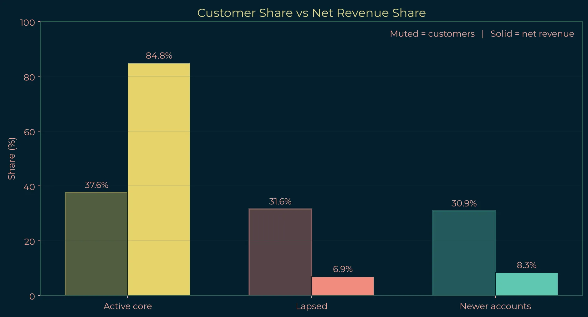
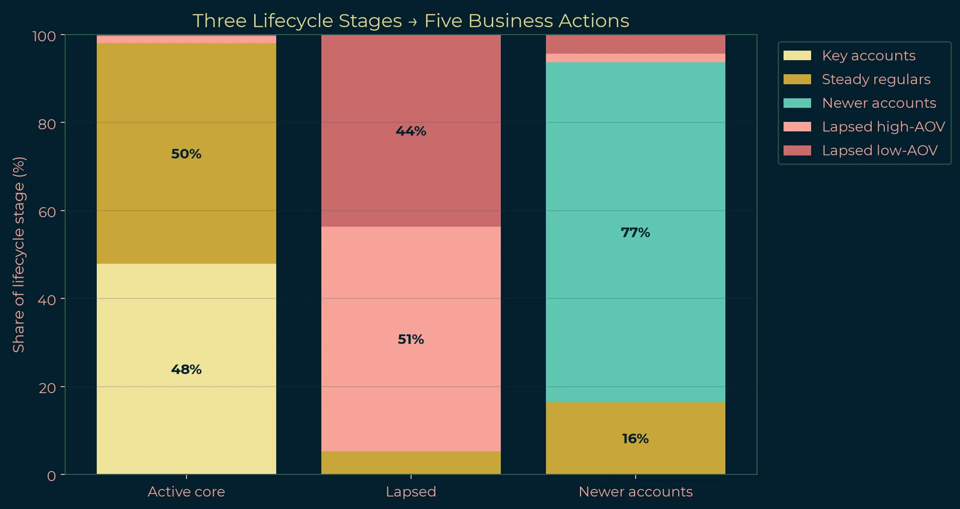
The primary k=3 solution divides 5,823 positive-net accounts into an Active core, Lapsed, and Newer accounts. The Active core contains 37.6% of accounts and produces 84.8% of net revenue. A secondary k=5 view turns those broad stages into a more operational segmentation: protect key accounts, grow steady regulars, convert newer accounts to another order, and distinguish high-value lapsed accounts from low-value ones before spending on win-back activity.
Data
Rebuilding account histories
The analysis uses the Online Retail II dataset from the UCI Machine Learning Repository, covering approximately 1.07 million transaction rows from a UK non-store retailer between December 2009 and December 2011. Many buyers are wholesalers, so CustomerID is treated here as an account identifier, not necessarily as an individual consumer (Chen, 2012). An earlier RFM segmentation study examined the same retailer's 2010–11 transactions (Chen, Sain & Guo, 2012).
Cleaning the transaction history
Exact duplicates were removed, records without usable account IDs were excluded from account-level modeling, nonpositive prices and known non-merchandise codes were handled explicitly, cancellations were reconciled against purchases, and all manual credits were subtracted from account spend under the final accounting policy. The reconciliation removed 1,210 same-day purchase-and-cancel pairs.
Two extreme cases show why that step matters. Account 12346 purchased and cancelled 74,215 units worth £77,183.60 within minutes; account 16446 did the same with 80,995 units worth £168,469.60. Keeping the purchase side while discarding the offsetting cancellation would manufacture two enormous high-value accounts.
Missing identifiers were also material. Records without an account ID represented 22.8% of deduplicated rows and 13.6% of gross line value. Those transactions remain outside the account-level clustering rather than being assigned artificially. After reconciliation and exclusions, the final table contains 5,823 accounts with positive net activity.
Method
Four features, two views
K-means clustering (MacQueen, 1967) uses four standardized account-level dimensions: recency, log frequency, log average order value, and observed tenure. Monetary value is not added as a fifth clustering feature because, in this account table, monetary value is exactly frequency × average order value; including all three would count the same purchasing information twice.
Selecting the primary solution
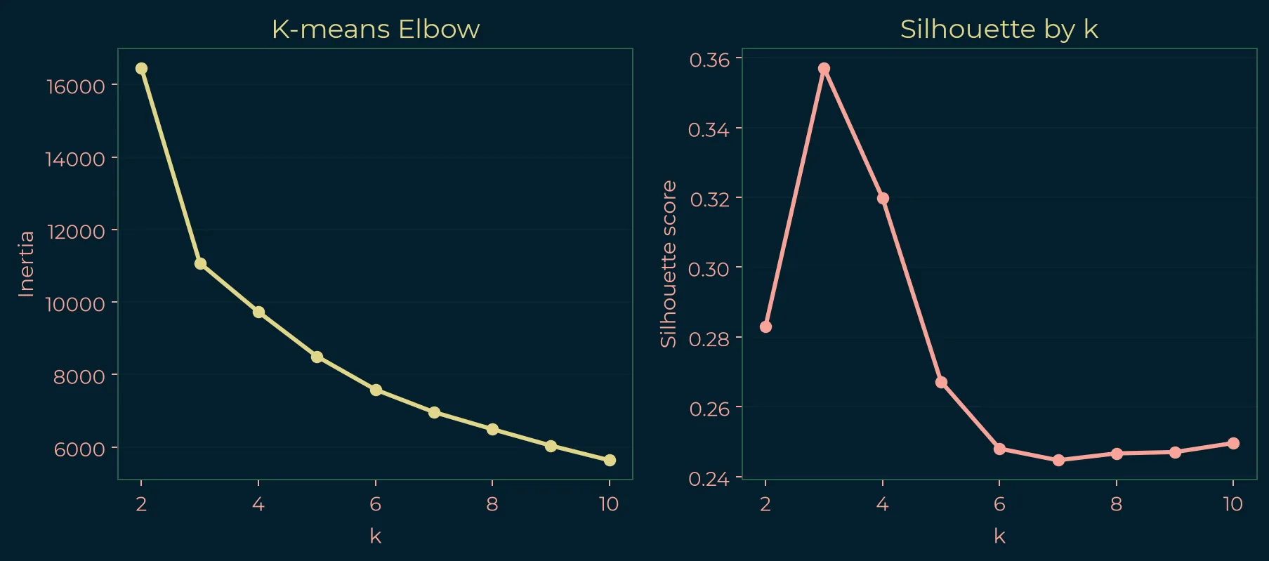
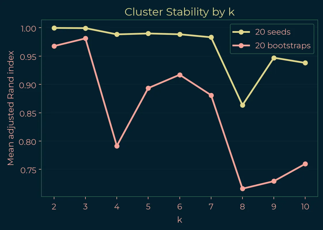
Solutions from k=2 through k=10 were compared using silhouette width (Rousseeuw, 1987), the Davies–Bouldin index (Davies & Bouldin, 1979), and the Calinski–Harabasz criterion (Caliński & Harabasz, 1974). Stability was tested by resampling after Hennig (2007) and measured with the adjusted Rand index (Hubert & Arabie, 1985).
The k=3 solution was strongest on the internal selection measures: silhouette ≈ 0.357, the lowest Davies–Bouldin score, the highest Calinski–Harabasz score, and bootstrap ARI ≈ 0.981. A Ward hierarchical comparison (Ward, 1963) produced ARI ≈ 0.56 against k-means, indicating useful structure without pretending that the boundaries are method-independent.
Why keep k=5?
The five-cluster solution is not presented as statistically superior to k=3. Its silhouette is 0.267 and its bootstrap ARI is 0.893. It is retained because it adds interpretable business detail while remaining materially more stable than k=4, whose bootstrap ARI is only 0.79. The result is a deliberate two-level interpretation: three lifecycle stages for the primary structure, five groups for action.
The manual-credit policy was also stress-tested. Under the alternative treatment, only 7 common accounts changed segment and the resulting k=3 assignments had ARI ≈ 0.996. The broad lifecycle result is therefore not being created by that accounting choice. The implementation uses scikit-learn (Pedregosa et al., 2011).
Results
Lifecycle first, action second
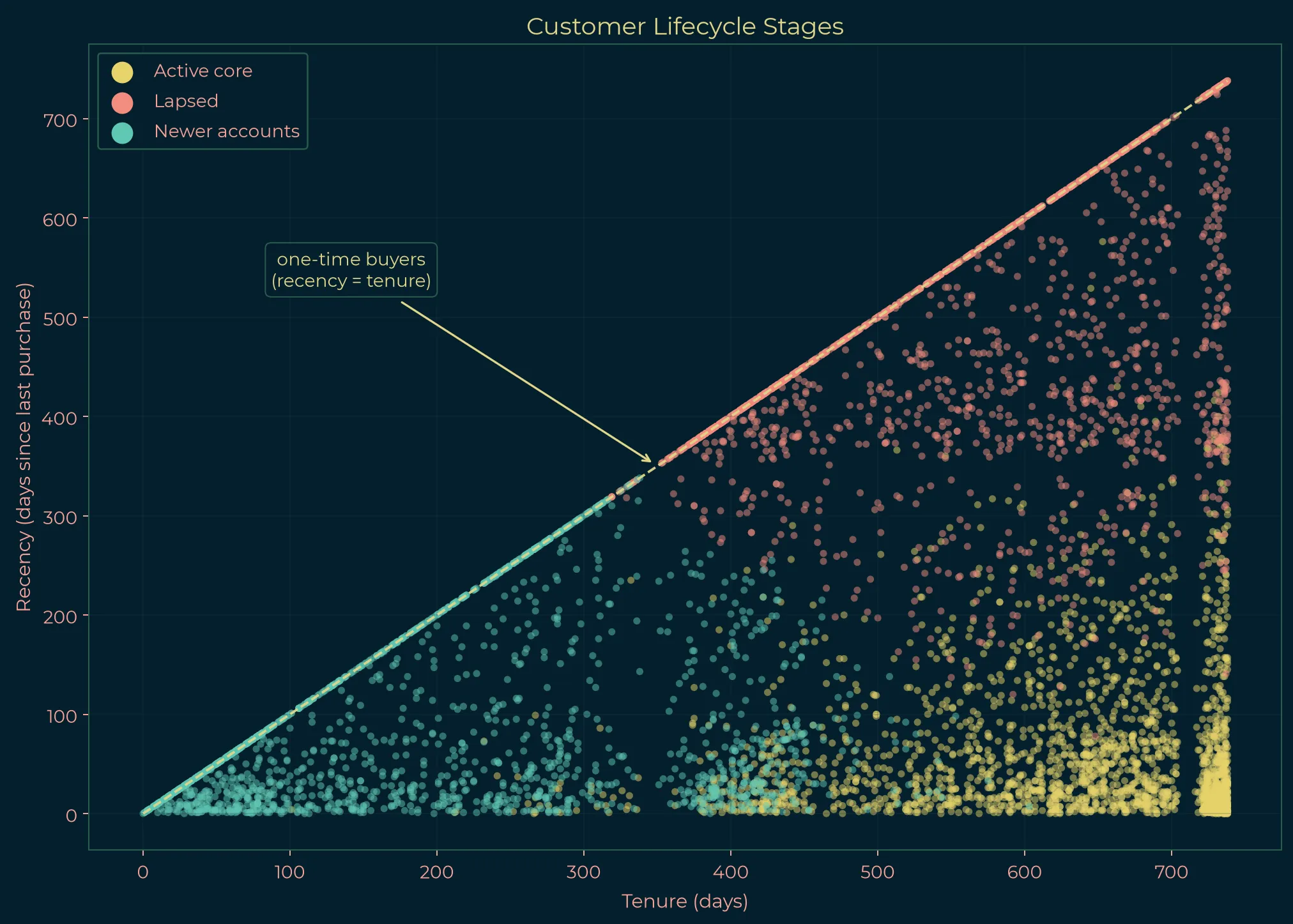
The k=3 solution separates accounts primarily by where they sit in the observed relationship. The Active core has a median tenure of 655 days. Newer accounts have a median tenure of 182 days. The Lapsed group is defined by long recency and low current activity, and 49.5% of those accounts are one-time buyers.
| Stage | Accounts | Share of accounts | Share of net revenue | Median tenure (days) |
|---|---|---|---|---|
| Active core | 2,188 | 37.6% | 84.8% | 655 |
| Lapsed | 1,838 | 31.6% | 6.9% | 574.5 |
| Newer accounts | 1,797 | 30.9% | 8.3% | 182 |
For a one-time account, recency and tenure are identical: its first observed purchase and most recent observed purchase are the same transaction. That identity creates the diagonal visible in the lifecycle scatter.
What tenure adds beyond RFM
RFM remains a useful way to summarize account value and activity (Fader, Hardie & Lee, 2005). But standard RFM has no tenure dimension. The k=3 Newer accounts span RFM scores from 4 through 15, overlapping established accounts with similar current recency, frequency, and monetary profiles. Tenure distinguishes accounts that are behaviorally similar now but are at very different stages of the observed relationship.
From three stages to five actions
The k=5 view refines the broad lifecycle structure rather than replacing it. Its Newer accounts group contains 1,390 accounts, compared with 1,797 in the k=3 Newer stage. Of those k=3 Newer accounts, 295 move into Steady regulars in the five-cluster view. The repeated name therefore refers to a narrower subset, not the identical population.
| Segment | Revenue position, Dec 2009–Dec 2011 | Action |
|---|---|---|
| Key accounts | 72.8% of net revenue | Retention and account management. Protect these first. |
| Steady regulars | 13.2% of net revenue | Grow order frequency. |
| Newer accounts (k=5) | 43.9% have ordered only once | Convert the account to a second order. |
| Lapsed high-AOV | £1.02M historical net revenue | Targeted win-back. |
| Lapsed low-AOV | £215k historical net revenue | Low-cost outreach or no outreach. |
The lapsed split makes the action logic concrete. Lapsed high-AOV accounts represent roughly £1.02 million in historical net revenue, compared with about £215,000 for the low-AOV group. Treating both as one generic lapsed audience would spend retention resources on accounts with very different historical value.
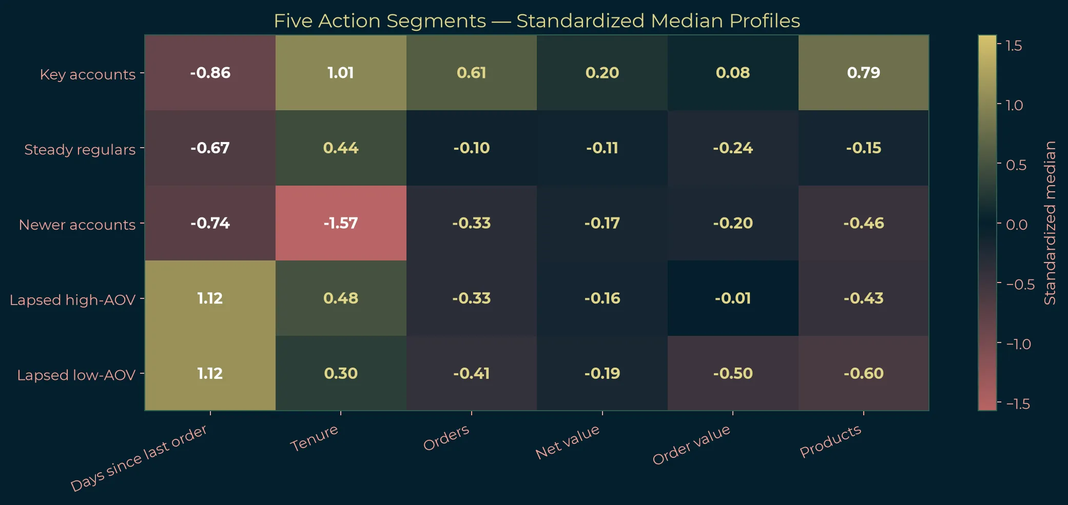
Three lifecycle stages. Five different actions.
Limits
Continuous structure, finite history
The clusters are useful boundaries on a largely continuous customer-lifecycle geometry, not sharply separated natural account types. A silhouette near 0.36 supports meaningful structure without implying clean islands, and the Ward-versus-k-means ARI of about 0.56 shows that some boundaries depend on clustering method.
Tenure is also observed tenure, not necessarily true relationship age. The dataset begins on 1 December 2009, so an account that was already active before the observation window can only be measured back to that boundary. Accounts at the maximum observed tenure of roughly 738 days therefore form the vertical band at the right edge of the scatter. “Newer” still means first observed well inside the window; the limitation applies mainly to interpreting the oldest accounts as having a precisely known start date.
The analysis is descriptive rather than predictive. It does not estimate future churn, lifetime value, or response to a specific intervention. In addition, 13.6% of gross transaction value cannot be linked to an account ID, and the data describe one retailer during 2009–2011. The segmentation therefore describes structure in this observed account base, not a universal retail taxonomy.
References
Sources
- Caliński, T., & Harabasz, J. (1974). “A dendrite method for cluster analysis.” Communications in Statistics, 3(1), 1–27. https://doi.org/10.1080/03610927408827101
- Chen, D. (2012). Online Retail II [Dataset]. UCI Machine Learning Repository. https://doi.org/10.24432/C5CG6D
- Chen, D., Sain, S. L., & Guo, K. (2012). “Data mining for the online retail industry: A case study of RFM model-based customer segmentation using data mining.” Journal of Database Marketing & Customer Strategy Management, 19(3), 197–208. https://doi.org/10.1057/dbm.2012.17
- Davies, D. L., & Bouldin, D. W. (1979). “A cluster separation measure.” IEEE Transactions on Pattern Analysis and Machine Intelligence, PAMI-1(2), 224–227. https://doi.org/10.1109/TPAMI.1979.4766909
- Fader, P. S., Hardie, B. G. S., & Lee, K. L. (2005). “RFM and CLV: Using iso-value curves for customer base analysis.” Journal of Marketing Research, 42(4), 415–430. https://doi.org/10.1509/jmkr.2005.42.4.415
- Hennig, C. (2007). “Cluster-wise assessment of cluster stability.” Computational Statistics & Data Analysis, 52(1), 258–271. https://doi.org/10.1016/j.csda.2006.11.025
- Hubert, L., & Arabie, P. (1985). “Comparing partitions.” Journal of Classification, 2(1), 193–218. https://doi.org/10.1007/BF01908075
- MacQueen, J. (1967). “Some methods for classification and analysis of multivariate observations.” In Proceedings of the Fifth Berkeley Symposium on Mathematical Statistics and Probability, Vol. 1, 281–297. https://projecteuclid.org/euclid.bsmsp/1200512992
- Pedregosa, F., Varoquaux, G., Gramfort, A., Michel, V., Thirion, B., Grisel, O., Blondel, M., Prettenhofer, P., Weiss, R., Dubourg, V., Vanderplas, J., Passos, A., Cournapeau, D., Brucher, M., Perrot, M., & Duchesnay, É. (2011). “Scikit-learn: Machine learning in Python.” Journal of Machine Learning Research, 12, 2825–2830. https://www.jmlr.org/papers/v12/pedregosa11a.html
- Rousseeuw, P. J. (1987). “Silhouettes: A graphical aid to the interpretation and validation of cluster analysis.” Journal of Computational and Applied Mathematics, 20, 53–65. https://doi.org/10.1016/0377-0427(87)90125-7
- Ward, J. H., Jr. (1963). “Hierarchical grouping to optimize an objective function.” Journal of the American Statistical Association, 58(301), 236–244. https://doi.org/10.1080/01621459.1963.10500845