Overview
Forecast Accuracy Depends on When You Look
The published EIA forecast is the most accurate model during the highest-demand hours, yet 84 percent of its net underforecast falls in nine daytime hours.
California electricity demand follows strong seasonal patterns across both the year and the day, but forecast accuracy is not uniform across time. A method that performs well at one forecast horizon or one hour of the day can perform very differently elsewhere.
This analysis uses hourly California regional demand from the U.S. Energy Information Administration’s EIA-930 dataset, spanning July 2015 through August 2026. It compares a 24-hour seasonal naïve forecast, Fourier terms with ARIMA errors, a fixed 50/50 average of those two forecasts, and the published EIA demand forecast.
The most unusual result is the behavior of the EIA forecast. It is highly accurate overnight and in the evening and performs best during the highest-demand hours, yet develops a large systematic gap during the middle of the day. Over the full evaluation window, it runs 2,845 MW below actual demand on average. The internally generated 50/50 ensemble produces the lowest overall MAE, but its advantage over the seasonal naïve forecast is about 11 percent under the broader four-origin evaluation, not the much larger advantage suggested by a single daily forecast origin.
Data
Eleven Years of Hourly Demand
The source is EIA-930, which publishes hourly demand and a day-ahead demand forecast for each balancing authority and for regions such as California (EIA, EIA-930 overview; EIA, Form EIA-930 instructions). The file contains 97,368 hourly rows. Twenty-four observations have missing demand values and were removed, leaving 97,344 observations in the working series. After those rows were removed, the hourly series contained no remaining gaps.
Figure 1 shows daily total demand across the full series. The recurring summer peaks are clear, but the source also contains 28 extremely low reported demand values concentrated in three distinct events.
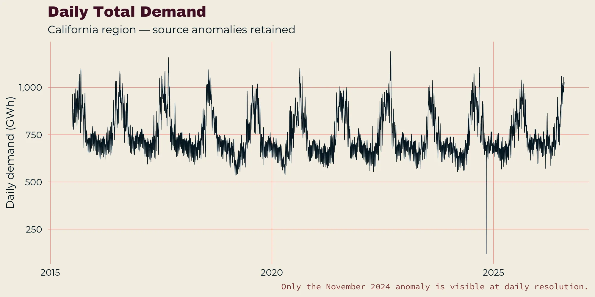
On November 5, 2017, one low observation occurs during the fall-back daylight-saving transition. On December 19, 2019, three consecutive hours report demand of roughly 6,000 MW while the published forecast remains near 30,000–35,000 MW. On November 2, 2024, reported demand remains near 4,000 MW for most of the day, while the EIA demand forecast follows the same unusually low level.
Those observations were retained rather than silently corrected or deleted. Their causes were not established. In particular, the balancing-authority components would need to be examined before attributing them to reporting, regional coverage, daylight-saving transitions, or another source issue. Only the full-history Fourier model could materially inherit these old observations, and this analysis did not separately test whether they affected its forecast accuracy.
Figure 2 shows average demand by month. Demand rises sharply into summer, with July and August producing the highest average loads.
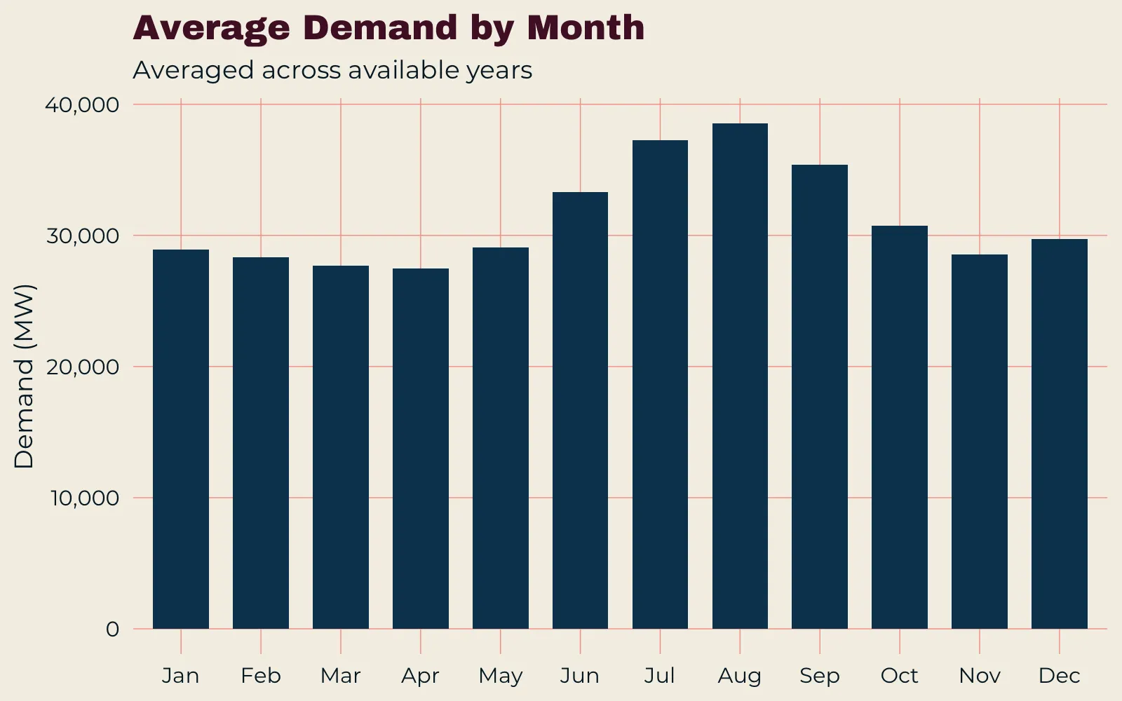
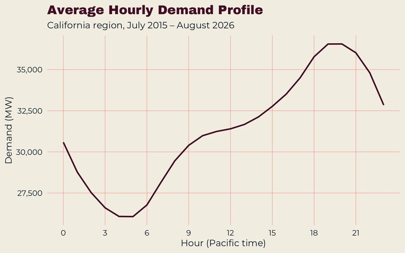
Figure 3 shows the average hourly demand profile in Pacific time. Demand reaches its minimum in the early morning and climbs toward a pronounced evening peak. This repeating daily shape is what the 24-hour seasonal naïve forecast exploits.
Method
Simple Models and a Published Benchmark
The evaluation uses the final 90 days of the available series, approximately mid-May through August 10, 2026. Accuracy is measured with mean absolute error (MAE) and root mean squared error (RMSE), both in megawatts (Hyndman and Koehler, 2006).
The primary baseline is a 24-hour seasonal naïve forecast, which predicts each hour using demand at the same hour one day earlier. A 168-hour version uses the corresponding hour one week earlier (Hyndman and Athanasopoulos, 2021).
The statistical model combines Fourier terms for daily and weekly seasonality with ARIMA errors, an approach suited to series with more than one seasonal cycle (Hyndman and Athanasopoulos, 2021). Univariate methods of this kind have been compared before for electricity demand up to a day ahead (Taylor et al., 2006; Taylor and McSharry, 2007). The specification uses:
- daily Fourier terms with K = 3
- weekly Fourier terms with K = 2
- fixed ARIMA(1,0,1) errors, with no automatic order search
- refitting at every forecast origin
Two training windows are compared. One uses all available historical data, while the other uses only the most recent 56 days.
A third forecast takes a fixed 50/50 average of the 24-hour seasonal naïve forecast and the 56-day Fourier + ARIMA forecast. Combining forecasts often reduces error relative to either input (Bates and Granger, 1969; Wang et al., 2023), and simple equal weights frequently outperform estimated weights, because estimating the weights adds error of its own (Smith and Wallis, 2009). The weights here are not estimated to minimize evaluation-period error.
The EIA benchmark
The published EIA demand forecast is included as an external benchmark. Each balancing authority produces it a day ahead for every hour of the following day (EIA, EIA-930 overview). Before scoring it, three timestamp alignments were tested. Matching the forecast and demand on the same row produced the lowest MAE at 2,995 MW. Shifting the forecast one hour forward increased MAE to 3,729 MW, while shifting it one hour backward produced 3,088 MW. The same-row alignment also produced a mean signed error of −2,845 MW, indicating systematic underforecasting during the evaluation window.
The large EIA error therefore does not appear to be caused by a simple one-hour timestamp mismatch.
Single-origin evaluation
One Forecast a Day Flatters the Statistical Model
The initial rolling-origin evaluation issues one 24-hour forecast per day at 00:00 UTC, refitting the models at each origin, and produces 89 completed forecast origins and 2,136 hourly forecasts (Tashman, 2000).
Under that design, the fixed 50/50 ensemble records an MAE of 1,427 MW, compared with 1,797 MW for the 24-hour seasonal naïve forecast and 1,803 MW for the trailing-56-day Fourier + ARIMA model. The same Fourier model records 2,232 MW MAE on the four-origin evaluation, showing that its single-origin score is strongly affected by when the forecasts are issued. The full-history Fourier model records 2,359 MW MAE; the analysis did not test why it performs worse.
The 168-hour seasonal naïve forecast performs substantially worse at 2,664 MW MAE, with a mean signed error of approximately −1,004 MW.
The larger ensemble advantage in this single-origin experiment should not be treated as the headline result. A 00:00 UTC origin places the earliest forecast horizons during Pacific evening hours, where the Fourier model happens to perform particularly well.
Failure modes
What the 14-Day Example Shows
Figure 4 illustrates why the models trade places. The Fourier + ARIMA forecast follows the broad daily rhythm but often remains too high during some of the deepest overnight troughs. The seasonal naïve forecast performs extremely well when consecutive days have similar shapes, but it can fail sharply when the next day differs from the one before it.
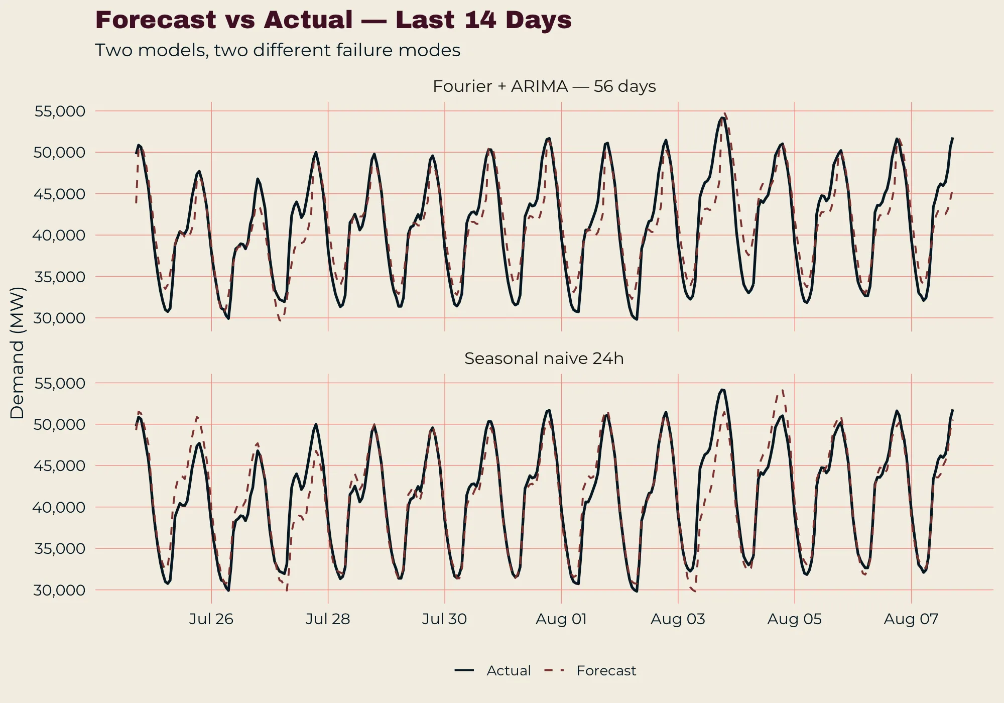
The figure is most useful as a view of those different failure modes. The aggregate MAE tables establish which method performs best overall; the 14-day window shows how those errors arise.
Multi-origin evaluation
Four Origins a Day Give a Fairer Comparison
To reduce the relationship between forecast horizon and hour of day, a second experiment issues forecasts four times per day at 00:00, 06:00, 12:00 and 18:00 UTC. This produces 356 completed forecast origins and 8,544 hourly forecasts.
| Model | MAE (MW) | RMSE (MW) |
|---|---|---|
| Naïve/Fourier 50/50 ensemble | 1,606 | 2,213 |
| Seasonal naïve 24h | 1,796 | 2,449 |
| Fourier + ARIMA, trailing 56 days | 2,232 | 3,063 |
| Published EIA forecast | 2,994 | 4,299 |
On this four-origin evaluation, which samples more of the day, the ensemble’s advantage over the seasonal naïve forecast is about 11 percent: 1,606 versus 1,796 MW. The larger single-origin gap reflects when those forecasts were issued: a 00:00 UTC origin places Fourier’s strongest horizons on the evening hours where it performs best.
The seasonal naïve model barely changes between the single-origin and four-origin designs: 1,797 versus 1,796 MW. Fourier changes from 1,803 to 2,232 MW. That contrast shows why the multi-origin result is the better summary of general model performance.
Forecast horizon
The Ensemble’s Advantage Is Front-Loaded
Figure 5 shows how forecast accuracy changes as the target moves farther from the forecast origin.
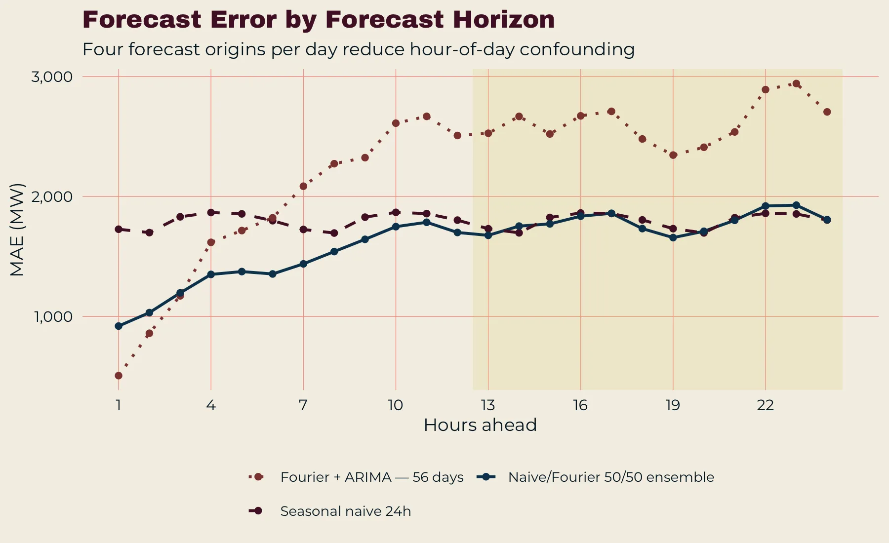
Fourier + ARIMA is best through the first three hours. At one hour ahead, its MAE is only 508 MW, compared with 921 MW for the ensemble and 1,727 MW for the seasonal naïve forecast. At two hours, Fourier remains best at 861 MW, and at three hours it records 1,173 MW versus 1,197 MW for the ensemble. The ensemble takes over at hour four.
By six hours ahead, Fourier has deteriorated to 1,822 MW, almost identical to the seasonal naïve forecast at 1,798 MW, while the ensemble remains lower at 1,355 MW.
The ensemble’s advantage is concentrated in roughly the first half of the forecast window. From 13 hours ahead onward, the ensemble and seasonal naïve forecast stay within about 75 MW of one another, and the ensemble is worse at six of those twelve horizons.
The horizon result is therefore more specific than “the ensemble wins.” Fourier contributes substantial information at very short horizons, the ensemble benefits from that information through roughly the first 12 hours, and beyond that point its performance is effectively the same as the seasonal naïve baseline.
Hour of day
The EIA Midday Gap
Figure 6 shows forecast MAE by Pacific hour. The ensemble and seasonal naïve forecasts are strongest overnight and early in the morning, with errors rising through the afternoon and peaking around 16:00–17:00. Fourier, not shown in the figure, is notably weaker than the ensemble overnight, at roughly 1,240–1,490 MW from midnight through 05:00.
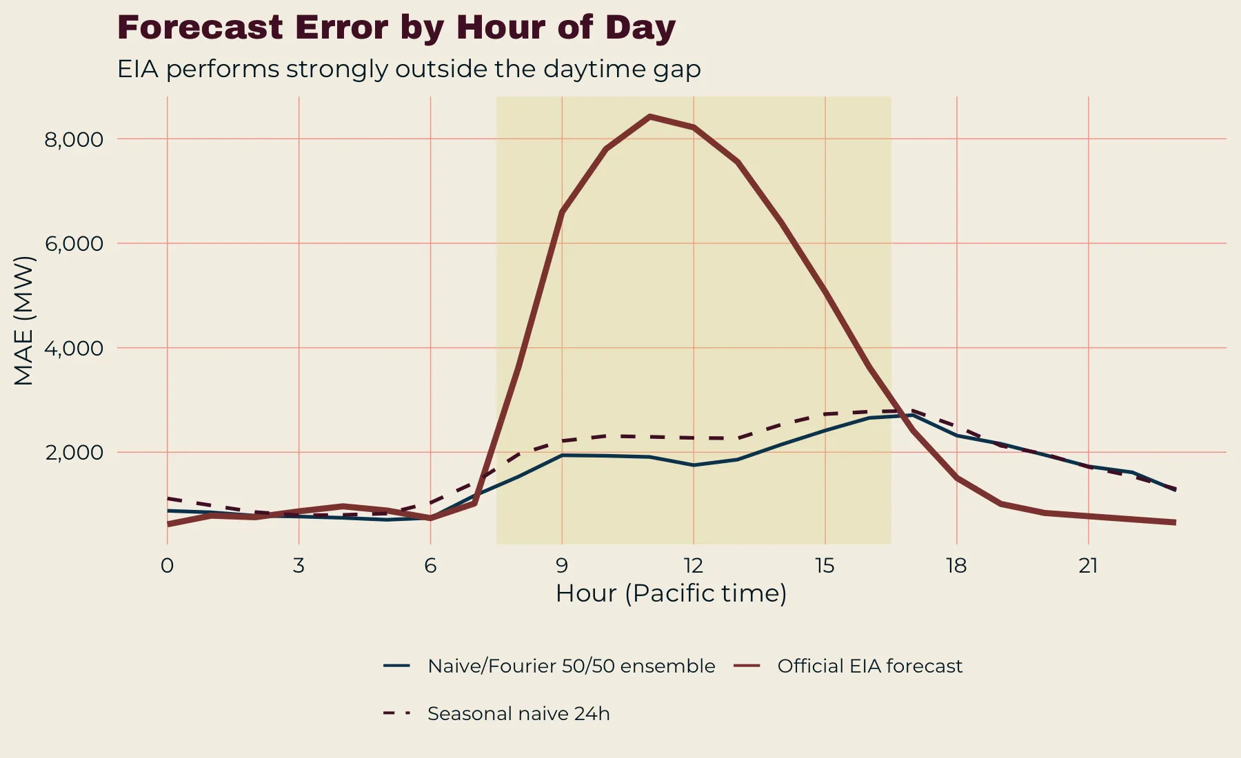
The EIA forecast behaves differently from the other models. It beats the ensemble in 12 of the 24 hours: 00:00–02:00, 06:00–07:00 and 17:00–23:00 Pacific. Its MAE is only 620 MW at midnight, 739 MW at 06:00, and 655 MW at 23:00.
From 08:00 through 16:00, however, its error increases dramatically.
| Pacific hour | EIA MAE (MW) |
|---|---|
| 08:00 | 3,616 |
| 09:00 | 6,599 |
| 10:00 | 7,806 |
| 11:00 | 8,424 |
| 12:00 | 8,218 |
| 13:00 | 7,557 |
| 14:00 | 6,391 |
| 15:00 | 5,070 |
| 16:00 | 3,632 |
Over the full window, the EIA forecast runs 2,845 MW below actual demand on average. Eighty-four percent of EIA’s net underforecast over the evaluation window occurs between 08:00 and 16:00 Pacific, nine hours that make up just over a third of the day. Its mean signed error is −6,370 MW during those hours, against −730 MW during the remaining fifteen.
The timestamp audit makes a simple one-hour alignment error unlikely, because both alternative shifts produce worse MAE. The analysis did not identify the cause of the gap. A definitional difference, publication process, regional aggregation issue, or another feature of the EIA series remains possible.
Peak demand
Peak-Demand Hours Tell a Different Story
The EIA forecast’s poor overall MAE hides one of the strongest results in the analysis.
In the single-origin evaluation, the 95th percentile of demand is 47,760 MW, leaving 107 hours in the top 5 percent group. During the other 95 percent of observations, the ensemble performs best at 1,395 MW MAE, while the EIA forecast records 3,062 MW.
During the top 5 percent of demand hours, however, the ranking reverses. EIA produces an MAE of 1,725 MW, compared with 2,024 MW for the ensemble and 2,187 MW for the seasonal naïve model. On the hours when load is highest, the official forecast is the strongest of the models tested.
That makes the EIA result more informative than its overall 2,995 MW MAE suggests. Its average score is dominated by a severe midday deficit, while its performance during peak-load conditions is comparatively strong.
Other results
Weekends and Daily Winners
Weekday and weekend
The weekday/weekend comparison also comes from the 89-day single-origin evaluation, so the weekend estimate rests on only roughly 25 weekend forecast days and should be interpreted accordingly. The ensemble records 1,495 MW MAE on weekdays and 1,244 MW on weekends. The recent Fourier model improves from 1,884 to 1,586 MW, while the seasonal naïve model moves in the opposite direction, increasing from 1,737 to 1,956 MW. The difference is descriptive rather than a separate large-sample result.
Daily winners
No model dominates every day. Across the 89 single-origin forecast days, the ensemble records the lowest daily MAE on 33 days, or 37.1 percent. The trailing-56-day Fourier model wins 19 days, the 24-hour seasonal naïve forecast 16, the 168-hour naïve 11, the full-history Fourier model 6, and the EIA forecast 4. The ensemble wins more days than any other model, but it does not win a majority.
Interpretation
One Average Hides the Important Behavior
The strongest result in the project is the EIA forecast’s hour-of-day structure. Its overall MAE is poor because of a pronounced daytime shortfall, yet it beats the ensemble during half of the clock hours and produces the lowest MAE during the top 5 percent of demand observations. That distinction matters because grid forecasting is not only about minimizing an average error across all hours; the most heavily loaded hours can matter disproportionately.
The ensemble remains the strongest internally generated forecast overall. Under the broader four-origin design it reduces MAE from 1,796 to 1,606 MW, about 11 percent, without estimating combination weights. But that improvement is concentrated in the first 12 hours. At longer horizons, the ensemble is effectively no better than the simple 24-hour seasonal naïve forecast.
Fourier + ARIMA provides the strongest short-range predictions but is much more sensitive to forecast timing. The seasonal naïve forecast is less impressive at the shortest horizons but remarkably stable across different forecast origins.
Together, these results show why a single overall MAE can obscure the most important forecasting behavior.
Limits
What These Results Do Not Support
The internally generated models use historical demand only. They do not include temperature, humidity, holidays, solar generation, or other exogenous variables commonly used in operational load forecasting (Fan and Hyndman, 2012; Hong and Fan, 2016).
The evaluation covers approximately mid-May through August 10, 2026, so the results primarily describe late-spring and summer conditions.
The four-origin design reduces but does not completely eliminate the relationship between forecast horizon and hour of day.
The 28 anomalously low observations were retained. Their causes were not established, the balancing-authority columns were not analyzed, and the effect of those observations on the full-history model was not separately tested.
Finally, the published EIA forecast is not necessarily based on the same information set or operational definition as the rolling models generated here. The analysis establishes the pattern present in the published series, not the reason that pattern exists.
Conclusion
Average Accuracy Is Not Operational Accuracy
The most consequential finding is that overall forecast accuracy and operationally important forecast accuracy are not the same thing.
The EIA forecast posts the worst overall MAE because of a large daytime deficit, yet it beats the ensemble during 12 of 24 hours and is the best-performing forecast during the top 5 percent of demand observations.
Meanwhile, a simple fixed 50/50 ensemble improves overall multi-origin MAE by about 11 percent relative to the 24-hour seasonal naïve model, with almost all of that advantage occurring during the first half of the forecast horizon.
Those results make the hour-of-day and peak-demand analyses more informative than a single leaderboard of average error.
Source
Repository
The analysis script, the EIA-930 source file, every output table and every figure are in the repository.
Sources
References
- Bates, J. M., and Granger, C. W. J. (1969). The combination of forecasts. Operational Research Quarterly, 20(4), 451–468. doi:10.1057/jors.1969.103
- Fan, S., and Hyndman, R. J. (2012). Short-term load forecasting based on a semi-parametric additive model. IEEE Transactions on Power Systems, 27(1), 134–141. doi:10.1109/TPWRS.2011.2162082
- Hong, T., and Fan, S. (2016). Probabilistic electric load forecasting: A tutorial review. International Journal of Forecasting, 32(3), 914–938. doi:10.1016/j.ijforecast.2015.11.011
- Hyndman, R. J., and Athanasopoulos, G. (2021). Forecasting: Principles and Practice (3rd ed.). OTexts. otexts.com/fpp3
- Hyndman, R. J., and Koehler, A. B. (2006). Another look at measures of forecast accuracy. International Journal of Forecasting, 22(4), 679–688. doi:10.1016/j.ijforecast.2006.03.001
- Smith, J., and Wallis, K. F. (2009). A simple explanation of the forecast combination puzzle. Oxford Bulletin of Economics and Statistics, 71(3), 331–355. doi:10.1111/j.1468-0084.2008.00541.x
- Tashman, L. J. (2000). Out-of-sample tests of forecasting accuracy: An analysis and review. International Journal of Forecasting, 16(4), 437–450. doi:10.1016/S0169-2070(00)00065-0
- Taylor, J. W., de Menezes, L. M., and McSharry, P. E. (2006). A comparison of univariate methods for forecasting electricity demand up to a day ahead. International Journal of Forecasting, 22(1), 1–16. doi:10.1016/j.ijforecast.2005.06.006
- Taylor, J. W., and McSharry, P. E. (2007). Short-term load forecasting methods: An evaluation based on European data. IEEE Transactions on Power Systems, 22(4), 2213–2219. doi:10.1109/TPWRS.2007.907583
- U.S. Energy Information Administration. About the EIA-930 data. Hourly Electric Grid Monitor documentation. eia.gov
- U.S. Energy Information Administration. Form EIA-930: Hourly and Daily Balancing Authority Operations Report, instructions. eia.gov
- Wang, X., Hyndman, R. J., Li, F., and Kang, Y. (2023). Forecast combinations: An over 50-year review. International Journal of Forecasting, 39(4), 1518–1547. doi:10.1016/j.ijforecast.2022.11.005