Overview
Congestion Is Not the Same as Breakdown
Three reasonable definitions of a traffic breakdown found 1,457, 10 and 7 events in the same four months of data.
A freeway can spend hours moving slowly without a new breakdown. It can also lose twenty miles per hour in five minutes and recover almost at once, or a queue can reach one detector while traffic a few hundred yards downstream is still moving normally. If the analysis begins and ends with a speed threshold, all of these look alike.
This project uses Caltrans Performance Measurement System (PeMS) data from February through May 2026 to study a five-station section of I-10 eastbound in District 7. PeMS collects loop detector data from California freeways and aggregates it into five-minute station records (Chen et al., 2001; PeMS field specification). The final corridor runs from the Vincent detectors through Lark Ellen to two stations near Azusa, about 1.2 miles in all.
I wanted to separate sustained congestion from the transition into it. From there the questions were what happens just before that transition, where it appears most often, how it spreads through the corridor, how long the resulting congestion lasts, and how it clears.
The analysis ended up using three related measurements: a sustained low-speed state, an abrupt speed collapse at a single station, and a spatial rule comparing neighboring stations. They produced very different event counts, and that difference became the starting point for everything that followed.
- 1,457Sustained congestion events
- 10Abrupt drops
- 7 of 10Drops that persisted
Data quality
The First Problem Was Deciding Which Measurements to Trust
Getting the data
PeMS distributes station data through its Clearinghouse as one compressed file per district per day, and each download requires a signed-in session. Four months of District 7 five-minute station data meant 120 daily files, about 2.2 GB in all, so I collected them with a Python script rather than by hand. The script read a list of Clearinghouse download links, kept only the files dated February through May 2026, and downloaded each one using the session cookie, pausing two seconds between requests to avoid loading the server. Each file was written to a temporary name and renamed only after it finished, so an interrupted run never left a partial file that looked complete, and files already on disk were skipped, so a run could be restarted where it stopped. Any download under 1 MB was rejected, since a real day of station data is far larger and a small file usually meant an error page instead of data. The script reported every failure at the end so missing days could be fetched again.
Coverage across the district
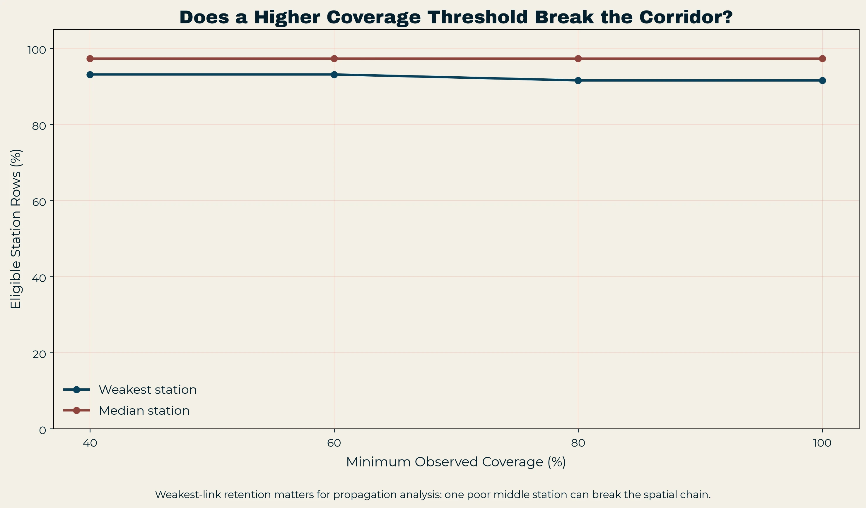
Before any events could be interpreted, the detector data needed to be checked. Across District 7 mainline stations, 85.8 percent of rows were 0 percent observed, and only 480 of 1,916 stations reported any observed data during the study period. Missing detector data in California is a long-standing problem: on a typical day in 2005, only about 60 percent of the statewide sensor network provided reliable measurements, and District 7 was among the weaker districts (Rajagopal and Varaiya, 2007). Coverage in 2026 was largely all or nothing, with almost no rows falling between 0 and 20 percent observed. The 480 reporting stations formed 31 contiguous runs of at least four adjacent stations. An early ranking favored a longer I-210 West run. The final selection ranked candidates by their weakest station’s coverage and by recurring low-speed traffic, and it chose this I-10 section.
PeMS reports a percent-observed value alongside speed, flow and occupancy. The field gives the percentage of individual lane points at a location that were observed rather than imputed (PeMS field specification). That distinction matters because PeMS detects bad or missing detector samples and fills them with values estimated from neighboring loops, producing a complete grid of data (Chen et al., 2003). A row with no observed coverage therefore does not appear empty. In this dataset, speed, flow and occupancy were often populated even when observed coverage was zero.
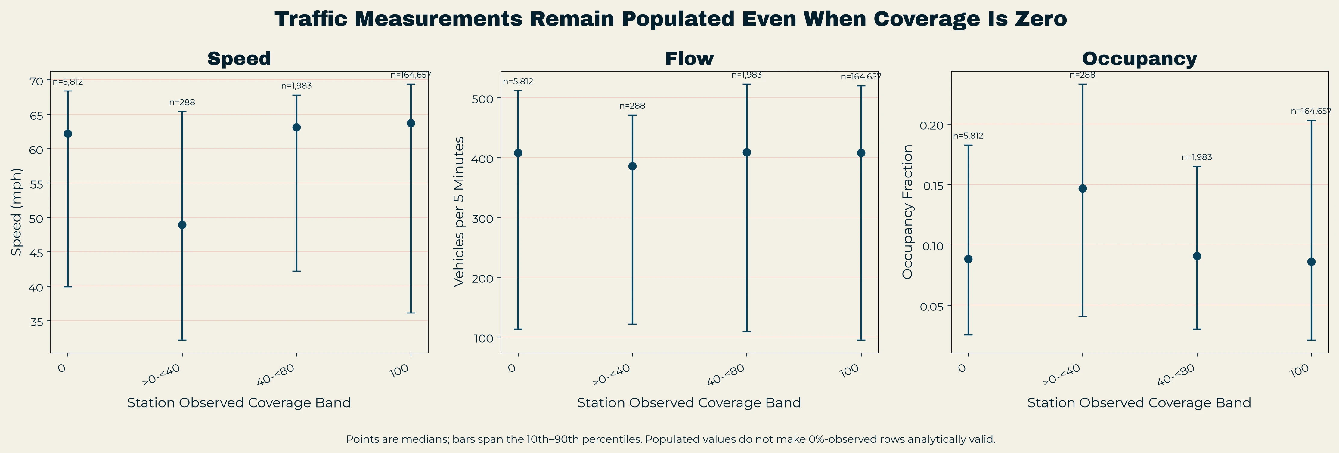
Figure 1 compares measurements across coverage bands. Speed, flow and occupancy are populated throughout the range, including the 0%-observed group, so the presence of a number in a measurement column does not show that the observation should be accepted. That is why the project filters on the coverage field instead of treating nonmissing speed or flow as evidence of a valid observation.
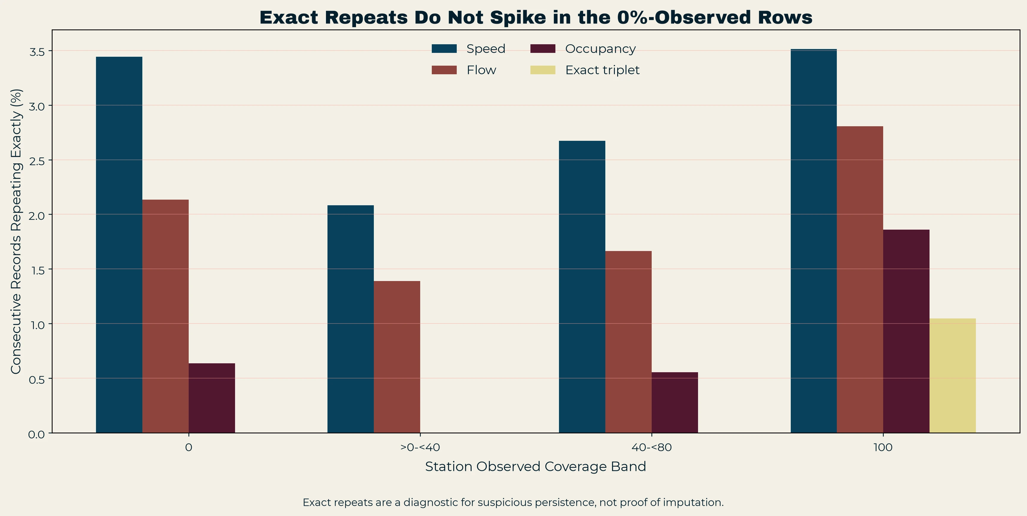
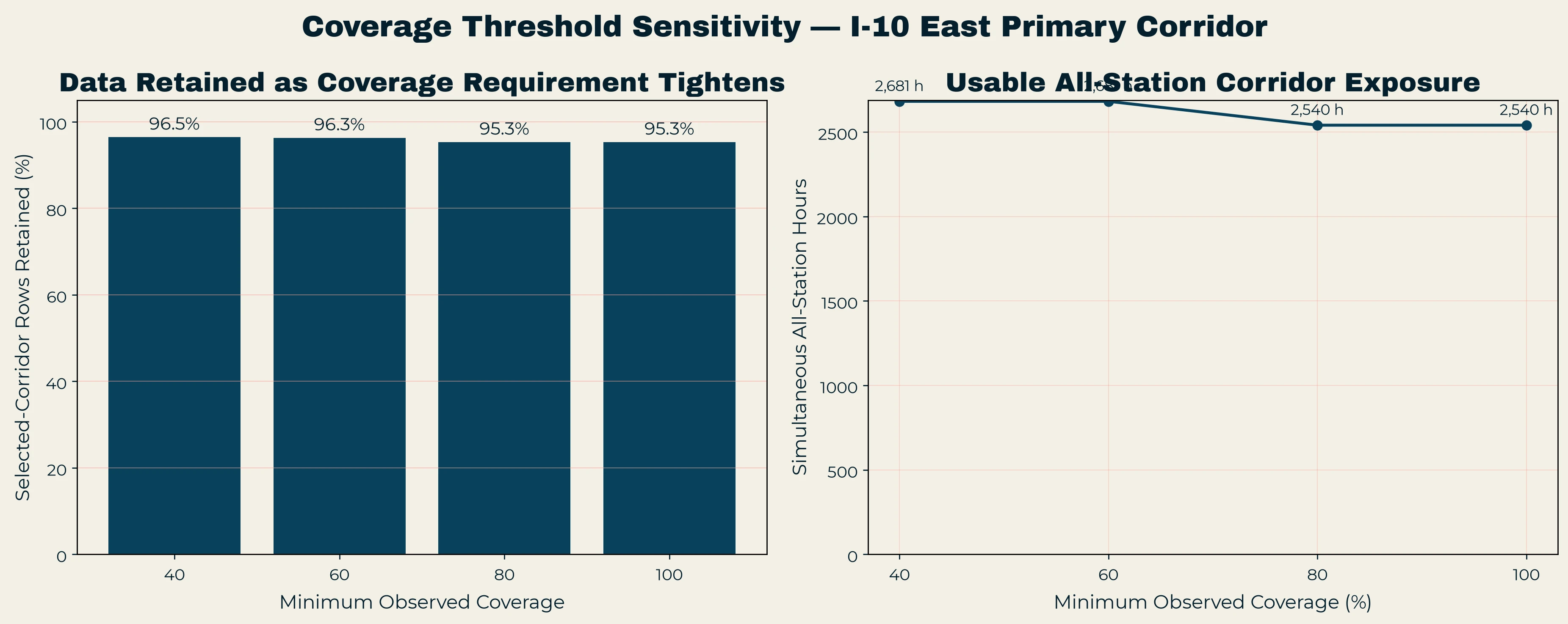
Three further checks shaped the sample. Values carried forward from the previous interval would be one explanation for populated rows at zero coverage, but the 0%-observed rows show no unusual rate of exact consecutive repeats (Figure A1). That does not establish where those values came from, but it rules out simple repetition. Station-level coverage also matched coverage calculated from the physical lanes listed in the station metadata exactly, so padded lane slots in the PeMS files were not distorting it. Finally, raising the minimum coverage requirement from 40 to 100 percent cost almost nothing on this corridor (Figure A2). Retained rows stayed near 95 percent, the 80% and 100% criteria produced the same final sample, and the weakest station stayed above 90 percent eligible rows even under the strictest requirement (Figure A3). A corridor analysis depends on its weakest station, since one unreliable detector can break the spatial chain no matter how good the median looks.
The final analysis therefore uses fully observed intervals on a five-station corridor with strong simultaneous coverage. These checks contain none of the headline findings, but they matter: a breakdown that appears because one station dropped out of the data is not a breakdown.
Event definitions
Three Definitions Produce Three Very Different Event Counts
The phrase traffic breakdown covers several possible measurements.
Sustained congested state
The simplest definition describes a sustained congested state. A station enters that state when speed stays below 50 mph for at least three consecutive five-minute intervals. FHWA treats 50 mph as an appropriate threshold for deciding when a freeway is congested, while noting that breakdown speeds vary from about 40 to 55 mph (FHWA-HOP-19-029). The three-interval minimum gives 15 minutes, the same persistence the Highway Capacity Manual requires before labeling conditions as level of service F (FHWA-HOP-08-054). This rule identified 1,457 events.
Abrupt drop
The second definition identifies an abrupt drop. Speed must fall by at least 20 mph from one five-minute interval to the next and finish below 40 mph. This rule was defined for this project. It adapts the 20 mph and 40 mph thresholds from Chen, Skabardonis and Varaiya’s Los Angeles work, where free-flow speed was near 60 mph and activated bottlenecks fell rapidly below 40 mph, to the change between consecutive intervals at a single station (Chen et al., 2004). The rule has no persistence requirement, so it can catch short-lived drops as well as lasting ones, which FHWA has also done in its own measures in order to capture transient breakdowns (FHWA-HOP-08-054). Ten events met this rule.
Caltrans spatial rule
The third definition follows the current Caltrans PeMS bottleneck documentation. It flags a location when the downstream station’s speed is below 40 mph, speed has dropped by at least 20 mph from the upstream station to the downstream station, the stations are less than 3 miles apart, and the condition holds in at least 5 of any 7 consecutive five-minute intervals (Caltrans PeMS). This rule runs in the opposite direction from the original PeMS bottleneck algorithm, which required the upstream detector to be below 40 mph and the downstream detector to be more than 20 mph faster (Chen et al., 2004). Seven events met the Caltrans rule. The classic pattern of a queue upstream and free flow downstream is examined separately later with a different measurement.
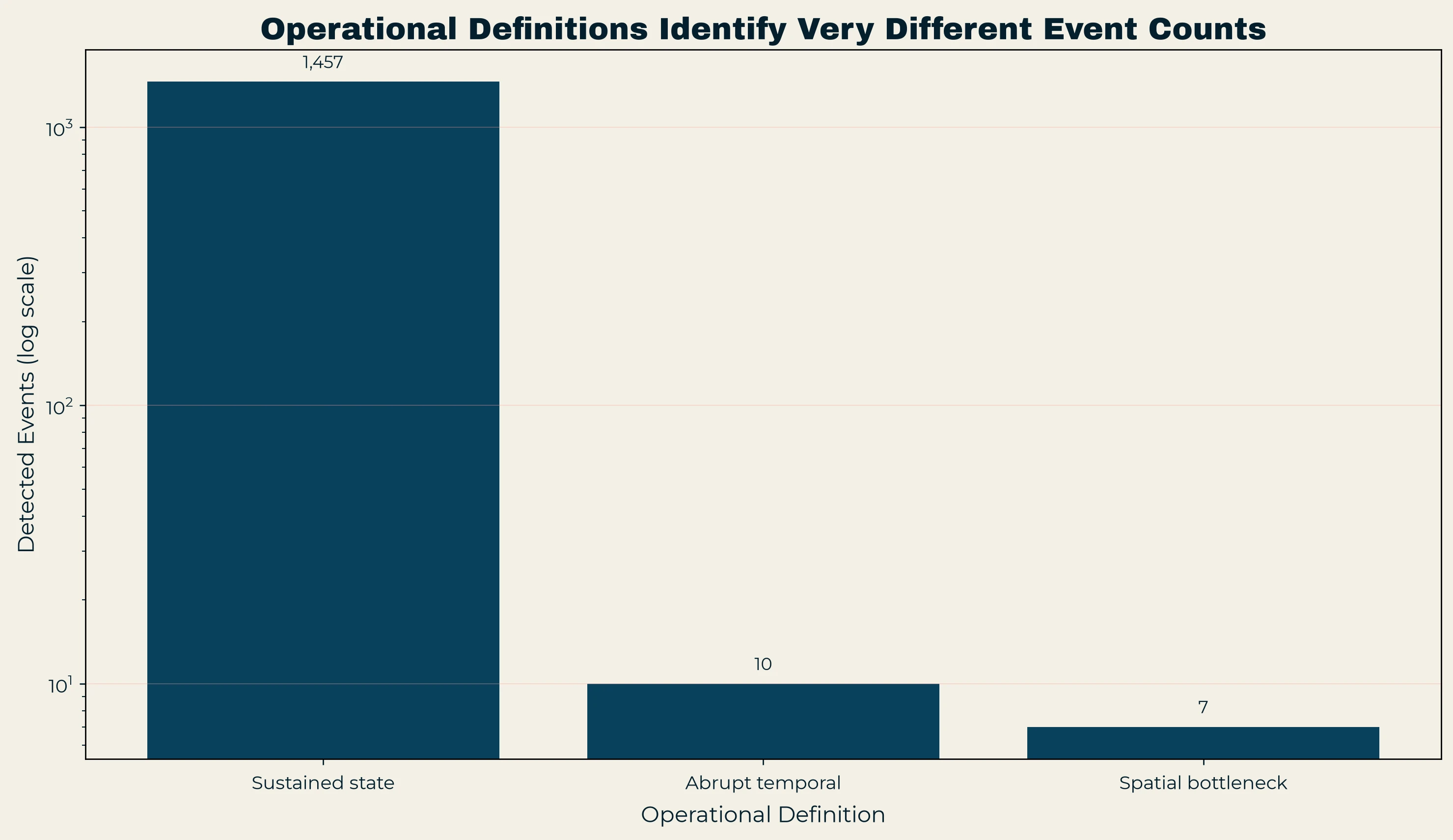
The counts are far enough apart that a linear chart would hide the smaller categories, so Figure 2 uses a logarithmic axis. The 1,457 sustained states, 10 abrupt drops and 7 Caltrans-rule detections are different event inventories. The sustained-state rule measures periods when low-speed traffic already exists, the abrupt-drop rule looks for the moment of a sharp collapse at one station, and the Caltrans rule looks for a particular speed relationship between neighboring stations. Calling all three “congestion events” would erase the reason for defining them separately. (The seven Caltrans-rule detections are unrelated to the seven persistent abrupt drops discussed below; the matching count is a coincidence.)
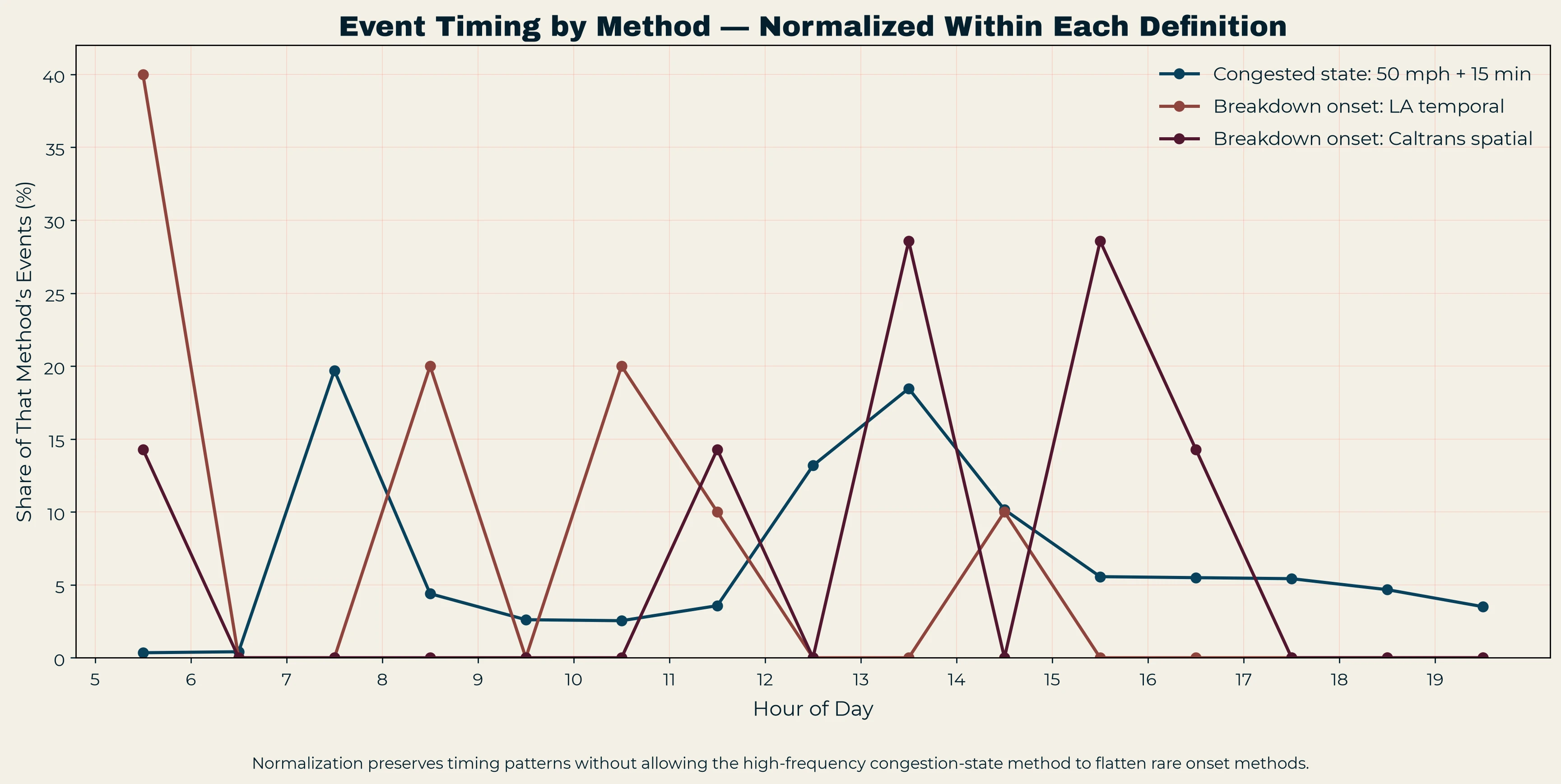
The timing distributions reinforce the distinction. Normalized by each method’s own event count, the profiles are not the same shape at different sample sizes (Figure A4). Sustained congestion covers a much broader part of the day, while the two onset rules are sparse and concentrated at particular hours.
That raises the question of whether the ten abrupt drops are ten equally convincing examples of a transition from free flow into sustained congestion, and on inspection they are not.
Event inspection
The Ten Abrupt Events Needed to Be Looked At Individually
The abrupt-drop rule is mechanical by design. A 20 mph loss ending below 40 mph either occurs or it does not, which makes the rule reproducible but does not make every detection the same kind of event.
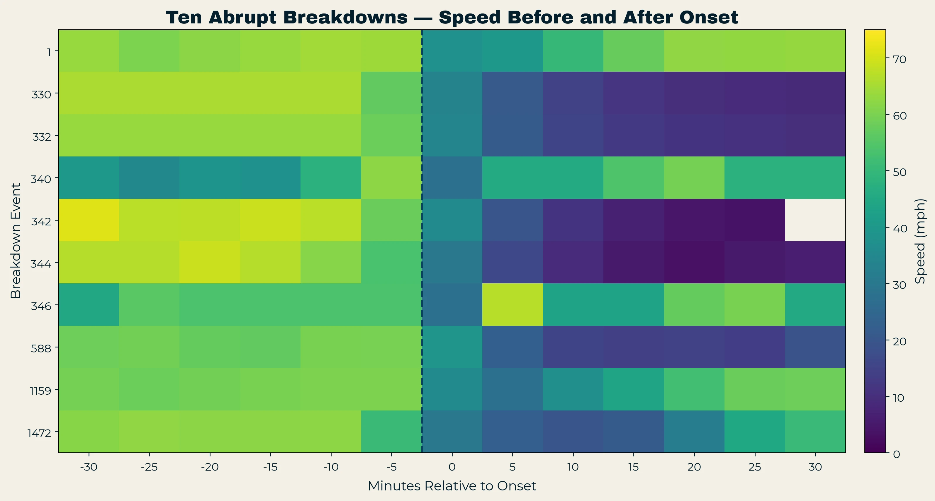
Figure 3 places all ten abrupt events on the same relative-time scale, from thirty minutes before onset to thirty minutes after. Most rows are fast before time zero and stay slow afterward, and the exceptions are easy to see.
Event 340 is the clearest exception on the pre-onset side. Traffic is already slow for much of the half hour before the detected drop. Speed rises to around 60 mph just before onset and then collapses again, so looking only at t−5 would label the event as a drop from free flow when the earlier observations show otherwise. Event 340 is at Azusa 2, the downstream-most station, on March 2. It is the same downstream-origin congestion that appears in Episode 3 below.
Events 1 and 346 raise a different problem. Their pre-onset conditions are consistent with free flow, but the low-speed state that follows does not last.
I checked persistence without replacing the original ten-event definition. Lorenz and Elefteriadou counted a speed drop as a true breakdown only when average speed stayed below their threshold for at least five minutes, to separate sustained breakdowns from short disturbances that the traffic stream absorbed (Lorenz and Elefteriadou, 2000, p. 89). Applying the same idea here, seven of the ten events remain below 40 mph at t+5, and the same seven remain below 40 mph through t+10. Events 1, 340 and 346 fail the check.
A wider pre-onset test takes the median speed from t−30 through t−10, requiring every five-minute interval in that window to be present. Nine of the ten events have a median above 50 mph. Event 340 is the exception, with a pre-window median of 38.7 mph. Events 1 and 346 have pre-window medians of 63.4 and 53.8 mph, so they begin in free flow but recover too quickly to meet the persistence check.
Event 1 sits exactly on one boundary. Its speed is 40.0 mph at t+5, while the check requires a value below 40. By t+10 it has risen to 50.3 mph, so treating 40.0 as inside or outside the threshold would not change its classification.
The result is a three-way split that leaves the primary definition alone. Seven events are sustained breakdowns beginning from free flow, two begin from free flow and behave as transient drops, and one is an abrupt deterioration inside traffic that was already congested. The ten-event inventory remains the primary sample because the rule was specified before this inspection. The seven-event group is a sensitivity subset, not a new definition chosen because it tells a cleaner story.
Pre-onset conditions
The Five Minutes Before Collapse Look Different
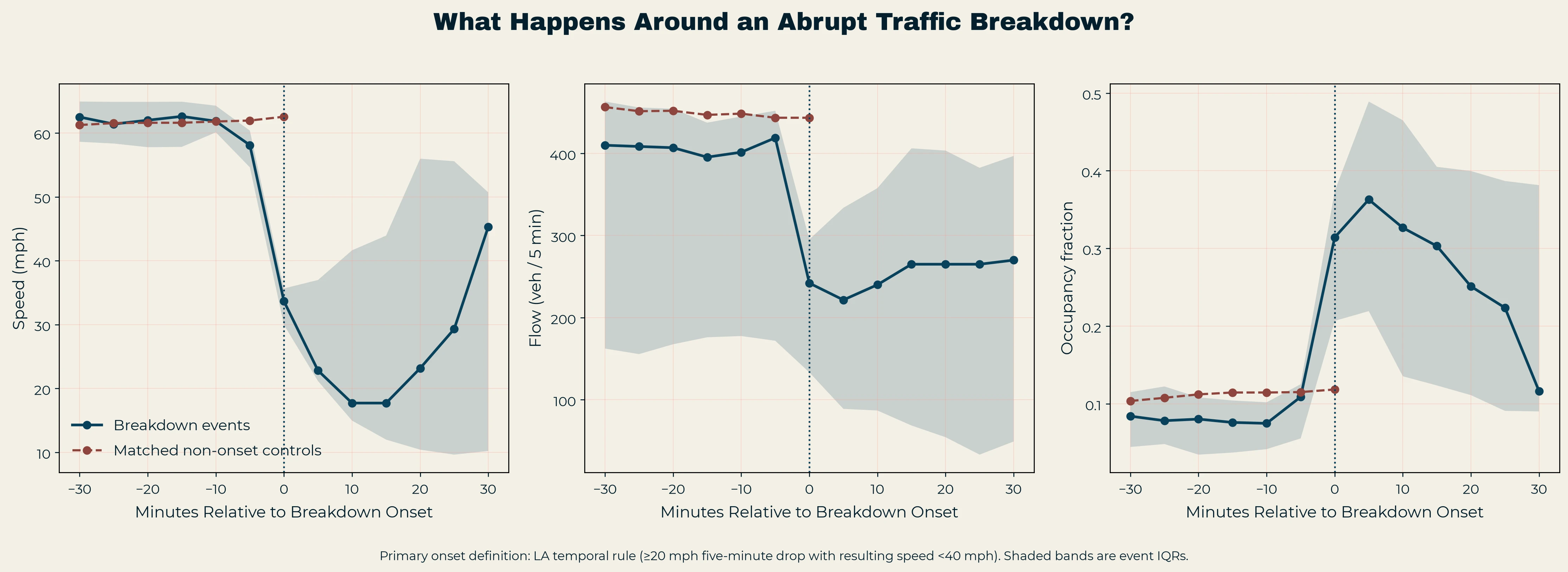
Figure 4 plots median speed, flow and occupancy around onset for the ten events. Speed is fairly stable before time zero, falls sharply at onset, and reaches its lowest values over the next several intervals before beginning to recover. Flow falls at the same time, and occupancy rises sharply as speed collapses.
The profile shows what happens around the events, but not whether the pre-onset values are unusual, which requires comparison periods. The first matched-control version allowed controls that were already congested. With those controls, event occupancy five minutes before onset was slightly lower than control occupancy, and the comparison looked weak.
The final control set matches station, day type and time of day while requiring speed above 50 mph at t−5, with ten controls for each abrupt event, 100 in all. Figure 5 shows the comparison at t−5. Median event speed is 58.1 mph against 63.0 mph for the free-flow controls. Median flow is 419 vehicles per five minutes for the events and 423.5 for the controls, so throughput is nearly identical. Median occupancy is 0.1088 for the events and 0.0873 for the controls. Just before the abrupt events, traffic is carrying about the same number of vehicles at a lower speed with more of the detector occupied.
| Median at t−5 | Abrupt events | Free-flow controls |
|---|---|---|
| Speed (mph) | 58.1 | 63.0 |
| Flow (veh / 5 min) | 419 | 423.5 |
| Occupancy | 0.1088 | 0.0873 |
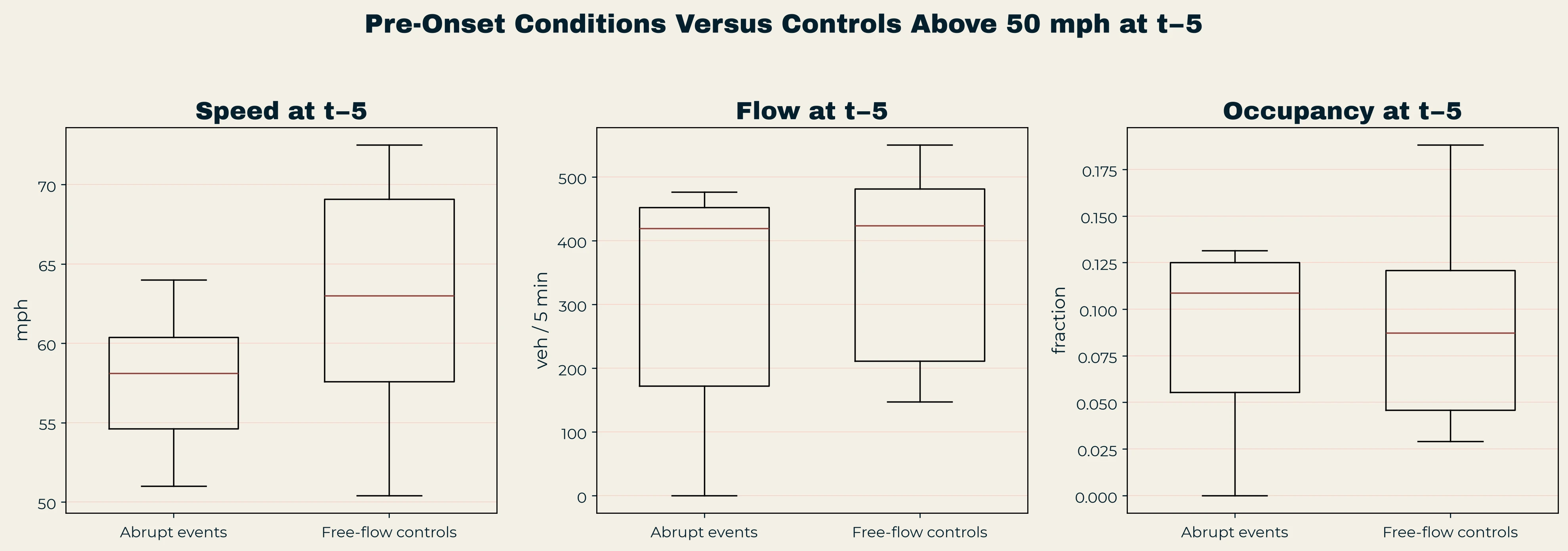
That pattern is consistent with density rising before the speed collapse. Chung, Rudjanakanoknad and Cassidy found that a pronounced increase in density always preceded the capacity drop at three freeway bottlenecks (Chung et al., 2007). Their density was measured over an extended roadway segment, while this project uses single-detector occupancy, so the result here agrees with theirs without measuring the same quantity. Chow, Lu and Qiu also modeled breakdown probability from the combination of incoming speed and occupancy and found that breakdown can occur while flow is below capacity (Chow et al., 2009), which fits a result where flow barely differs and speed and occupancy do.
The earlier control set hid this because already-congested comparison intervals pushed control occupancy upward. Restricting the controls to free-flow observations reversed the comparison.
The timing within the event group adds another piece. Median occupancy for all ten events rises from 0.0747 at t−10 to 0.1088 at t−5. For the seven persistent events it rises from 0.0804 to 0.1239. The data do not show a gradual thirty-minute buildup. Conditions can look ordinary ten minutes before onset and much denser five minutes later.
A five-minute value averages everything inside the interval, and averages taken from fixed consecutive intervals during changing conditions need not describe a stable traffic state (Cassidy, 1998). If the collapse began partway through the t−5 interval, that interval would already show higher occupancy and lower speed. These data cannot separate “density rose before breakdown” from “breakdown started inside the t−5 window.”
None of this provides a forecasting rule. Ten events are too few, and the distributions overlap: at t−5 the event occupancy interquartile range is roughly 0.055 to 0.125, and the free-flow control range is roughly 0.046 to 0.121. Breakdown is also probabilistic. Flows well above queue discharge rates do not always produce a breakdown (Persaud et al., 1998), so a single threshold value would not be expected to separate events from controls. The supportable result is narrower: in these ten events, the final interval before onset had lower speed and higher occupancy than matched free-flow observations at nearly the same flow. The difference is larger for the seven persistent cases, but the full ten-event sample remains the primary analysis.
Spatial pattern
A Recurring Bottleneck Between Lark Ellen and Azusa 1
The abrupt-drop rule asks when speed collapses at one station. A separate question is where in the corridor the classic bottleneck pattern appears. An active bottleneck is commonly described as a location with queued traffic upstream and free-flowing traffic downstream (Daganzo et al., 1999; FHWA-HOP-18-013).
I checked each pair of adjacent stations for that pattern. A pair counted when the upstream station was below 50 mph while the downstream station stayed at or above 50 mph, and pairs were ranked by how many times that pattern persisted for at least 15 minutes. This follows the direction of Chen et al. (2004), but with a 50 mph threshold at both stations rather than Chen’s criteria of upstream speed below 40 mph and a gap of more than 20 mph (Chen et al., 2004). The top pair was Lark Ellen (716152) to Azusa 1 (717195), with 172 persistent runs against 36 for the next pair. That fits a long line of findings that freeway bottlenecks occur at fixed, reproducible locations (Cassidy and Bertini, 1999), and a similar PeMS-based study on I-405 in Orange County located repeated bottleneck activations along a six-mile segment using the same upstream-queued, downstream-unqueued logic (Bertini and Myton, 2005).
- 172Persistent runs, Lark Ellen → Azusa 1
- 36Next-highest pair
The duration results point the same way. The three stations upstream of this pair (Vincent 1, Vincent 2 and Lark Ellen) have median congestion durations near 80 minutes, and the two downstream of it are near 50. That is what a queue building upstream of a bottleneck and discharging past it would produce.
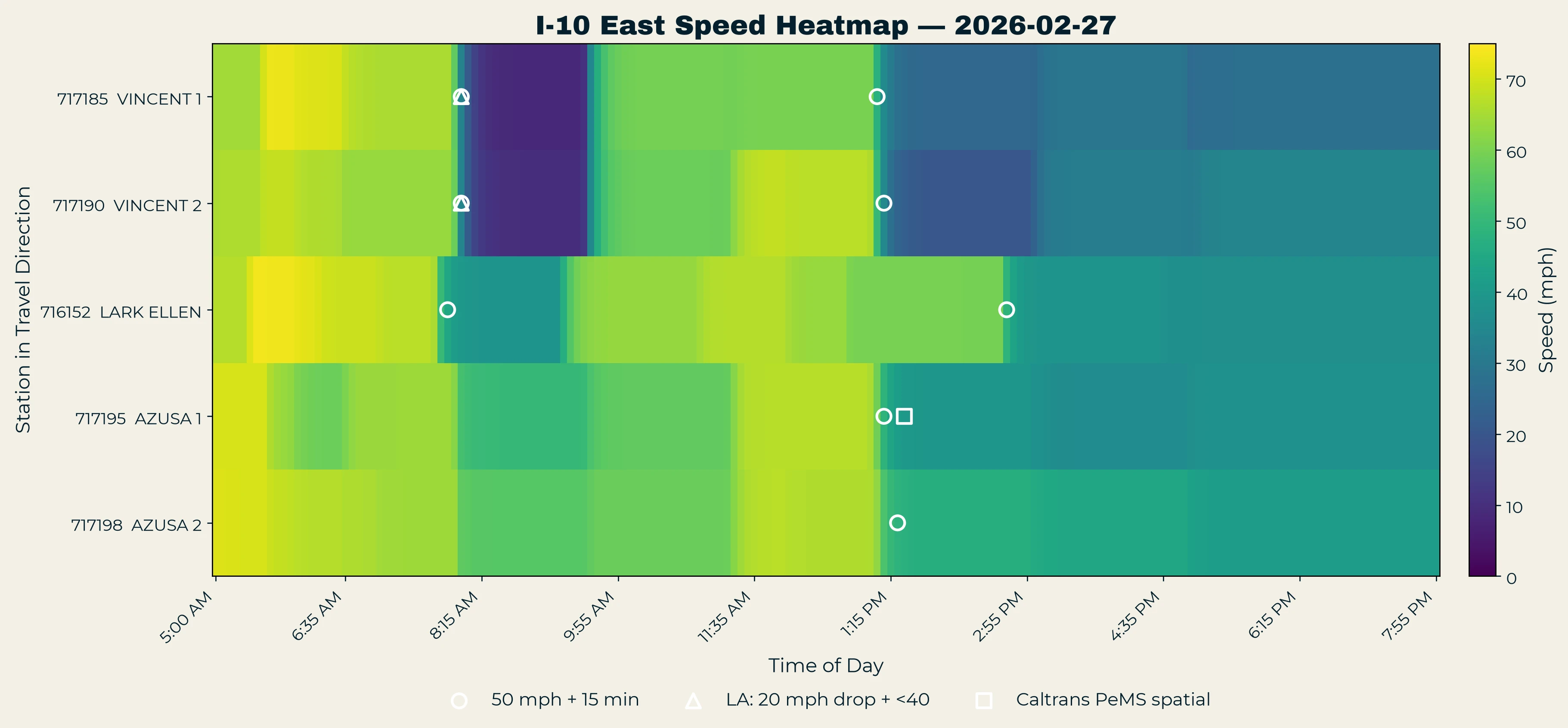
Figure 6, built around February 27, shows all five stations through the day with markers for the different event definitions. The abrupt-drop and Caltrans-rule markers do not land on the same coordinates, and at several times the heatmap shows a sharp change from one detector to the next rather than a corridor-wide collapse. A station-by-station time series cannot show that relationship.
The corridor is only about 1.2 miles long, so this places a recurring bottleneck inside the observed section without showing that every disturbance starts there. Episode 3, described below, appears to enter from the downstream boundary instead, and its initiating conditions may have developed beyond the last detector. The seven events from the Caltrans PeMS rule measure a different pattern and are not part of this ranking.
Corridor episodes
Ten Station Events Became Six Corridor Episodes
The abrupt-drop rule works at the station level, so several stations can record related onsets during the same traffic episode. Grouping the ten detections by date gives six episodes. Because the grouping is by day, the six episodes are simply six calendar dates, so I make no claim that the events cluster in any more general sense.
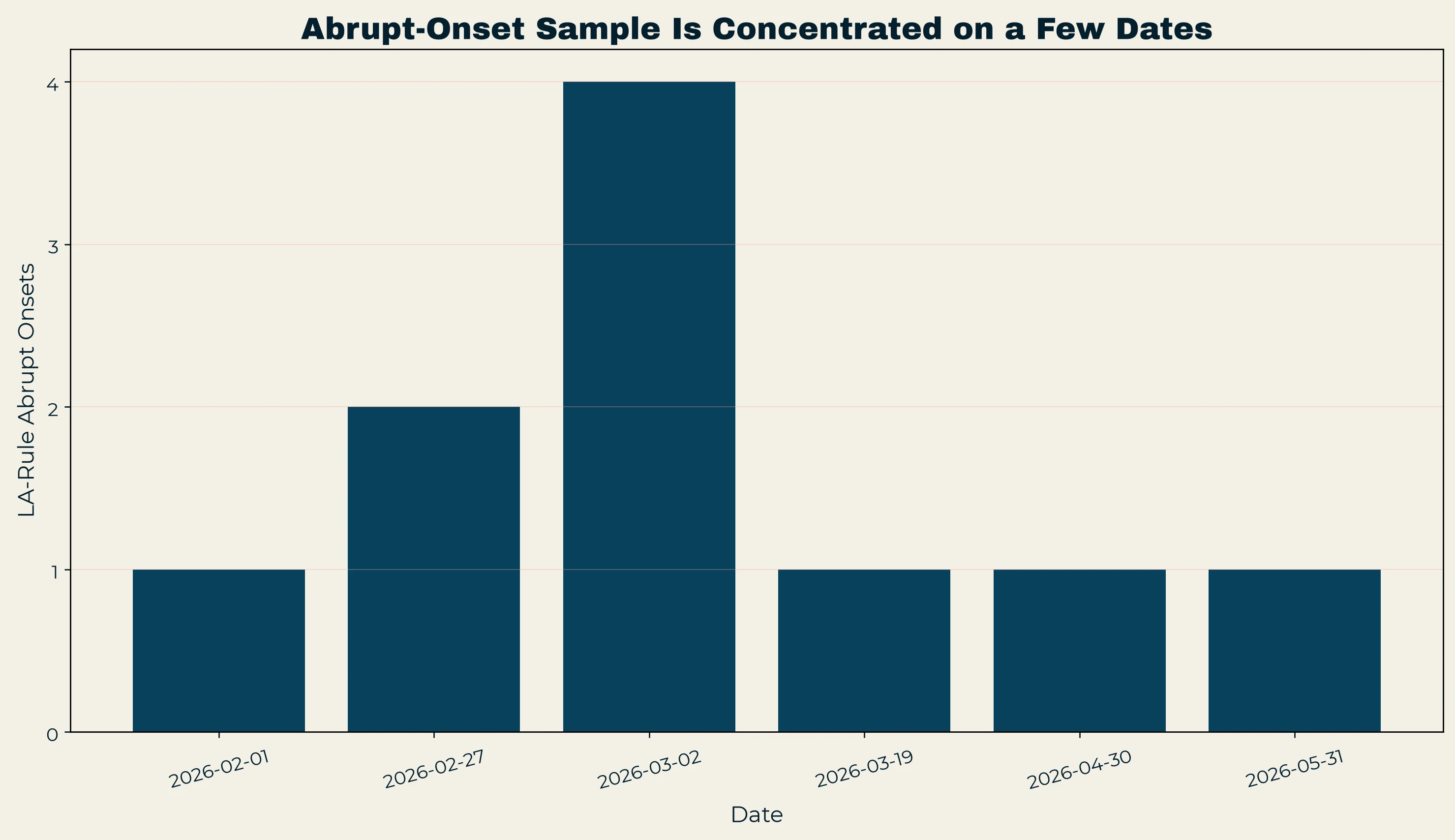
The dates are uneven (Figure A5): four of the ten abrupt onsets occurred on March 2, two on February 27, and four other dates contributed one event each. Four March 2 detections are not four independent days of evidence, and that concentration limits any analysis built on ten events. I did not assign a cause to the March 2 cluster; the analysis does not identify an incident, weather condition or other external explanation.
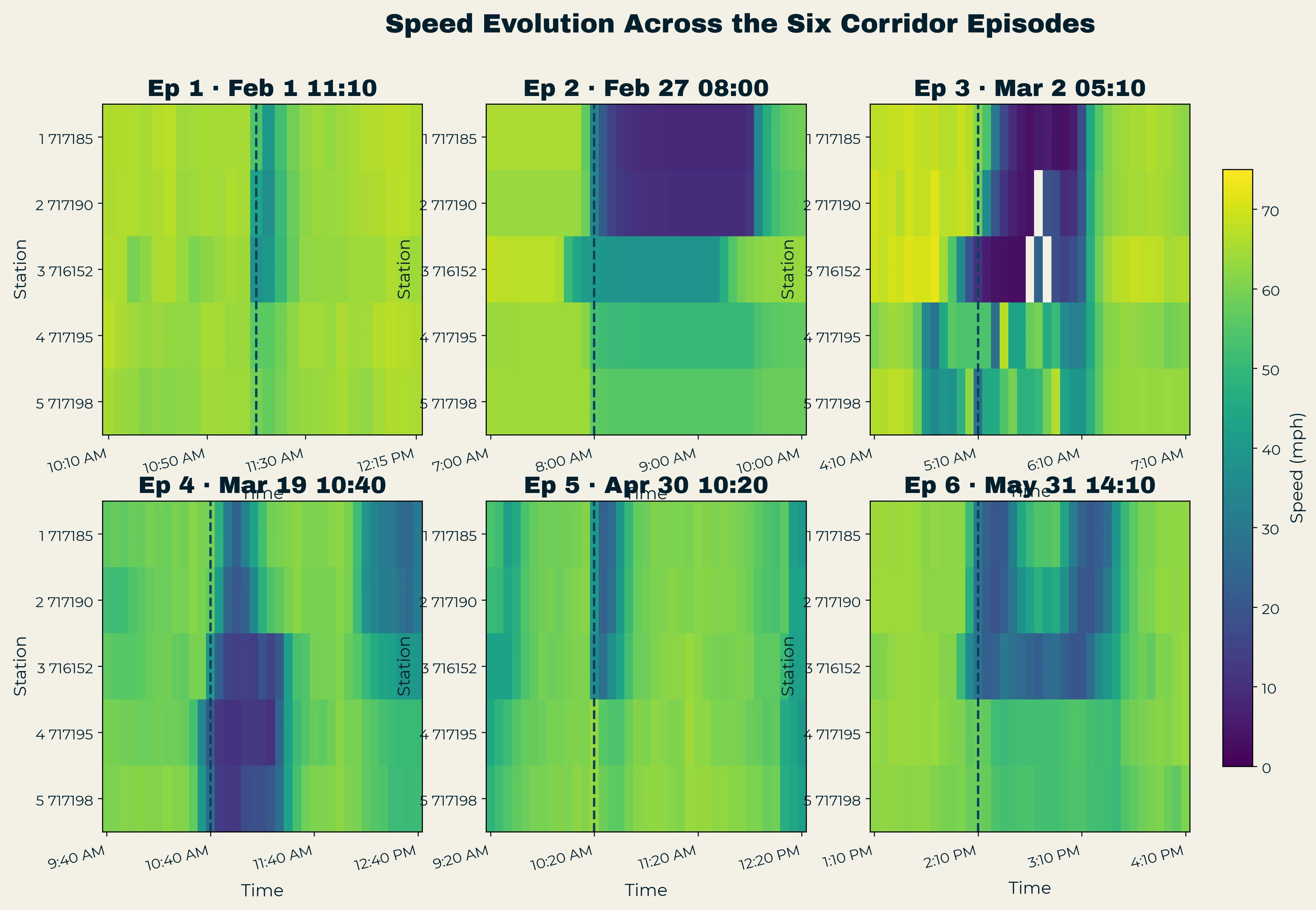
Figure 7 places all six episodes in a common grid, with each panel showing speed across the five stations before and after the first abrupt onset. The panels do not look like six copies of one template. Episode 1 stays fairly localized, and Episode 2 shows a stronger multi-station deterioration. Episode 3 is the largest cluster, with four station-level detections, and its first visible deterioration is at the downstream end of the corridor, where event 340 sits. That is the main reason I would not claim the full initiation process was observed. Episode 4 develops into a broad low-speed state across the corridor, Episode 5 spreads more slowly, and Episode 6 involves several stations without a simple end-to-end wave. The grid describes the variation better than any single propagation statistic would.
Propagation
Propagation Depends on How Long You Wait
I measured the delay between the first abrupt onset in each episode and the time each station entered sustained congestion. In traffic flow theory, the boundary between congested and uncongested traffic moves along the road as a wave (Lighthill and Whitham, 1955), so the order in which stations enter congestion says something about where that boundary travels.
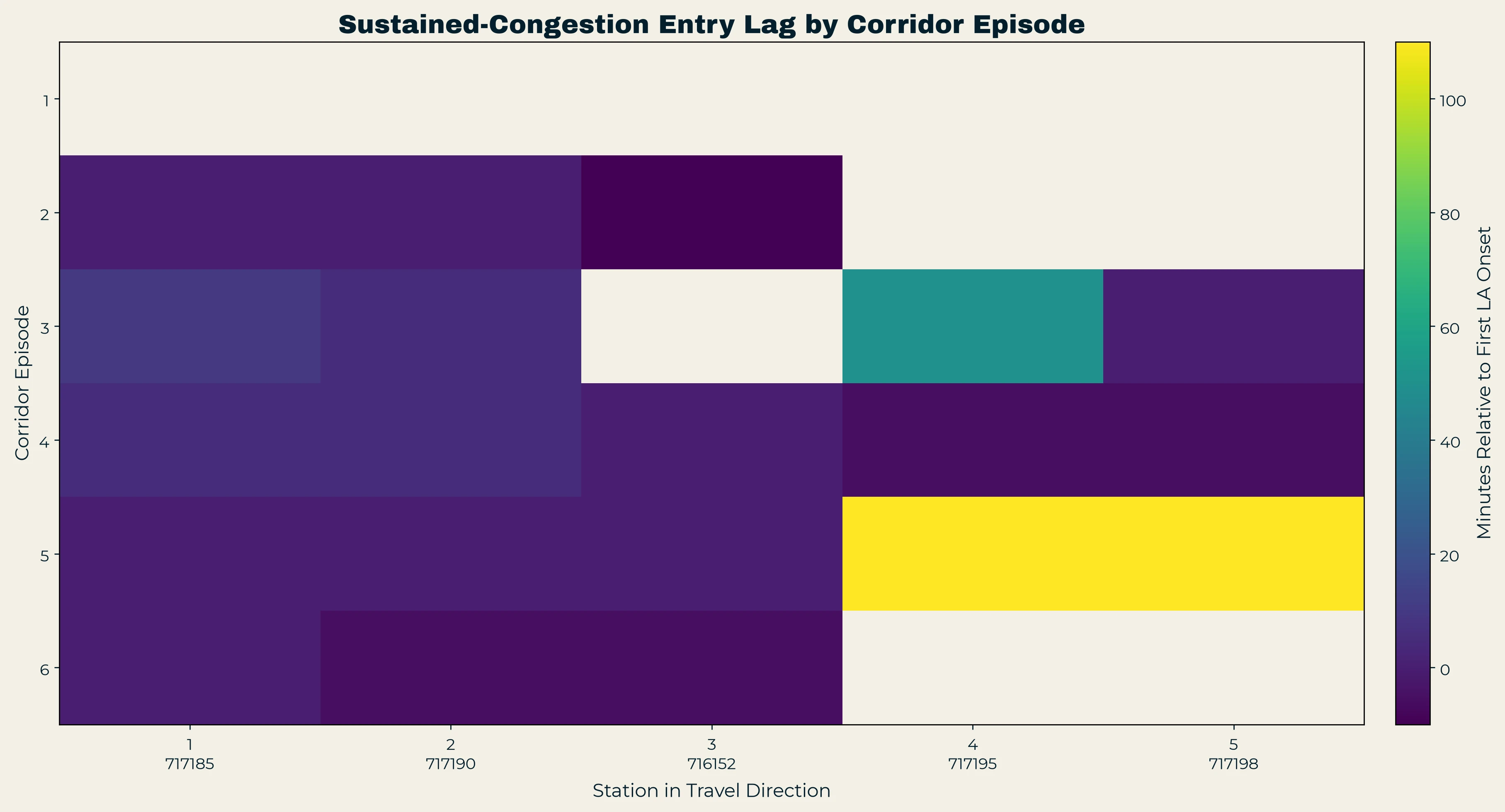
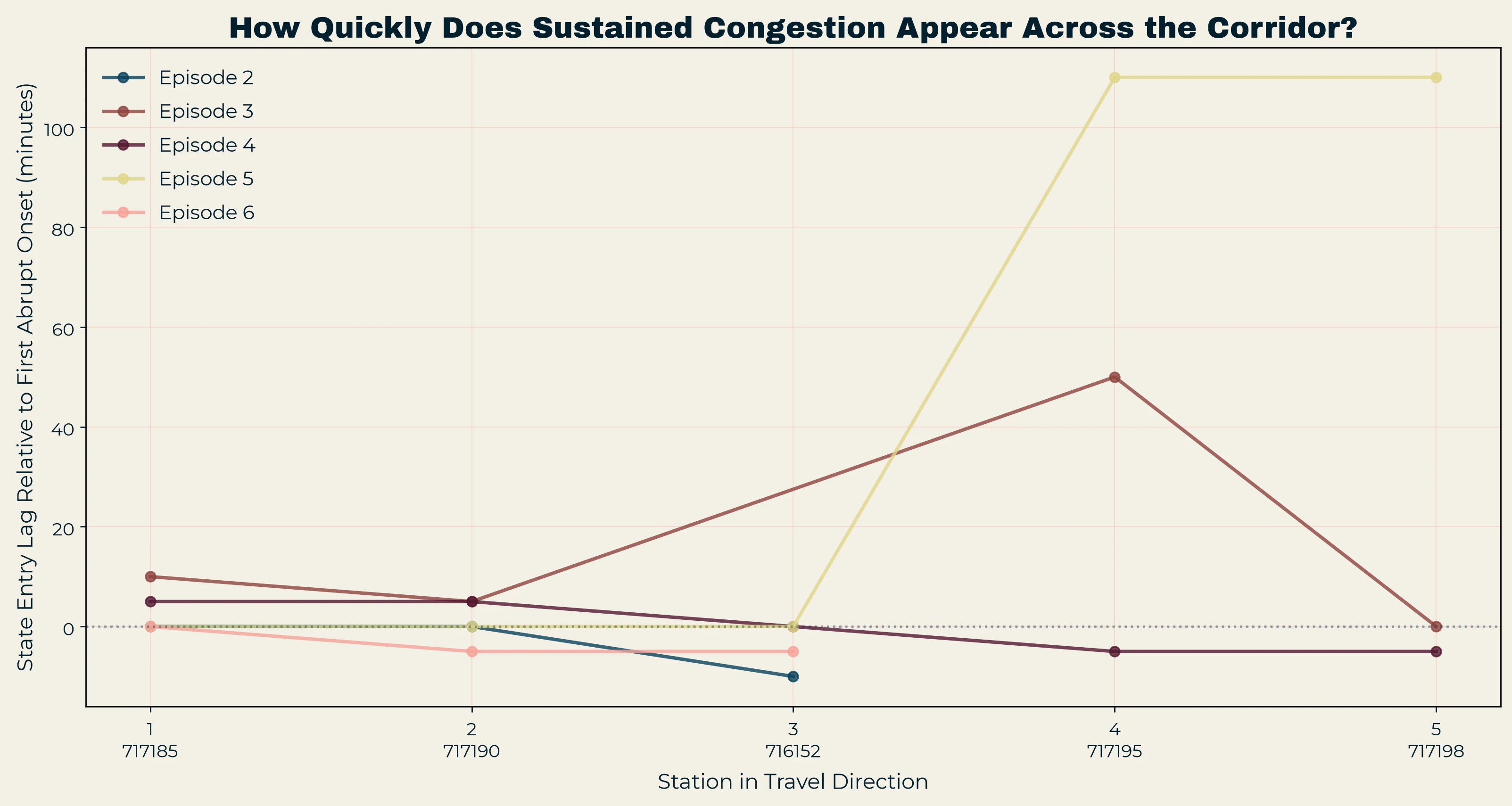
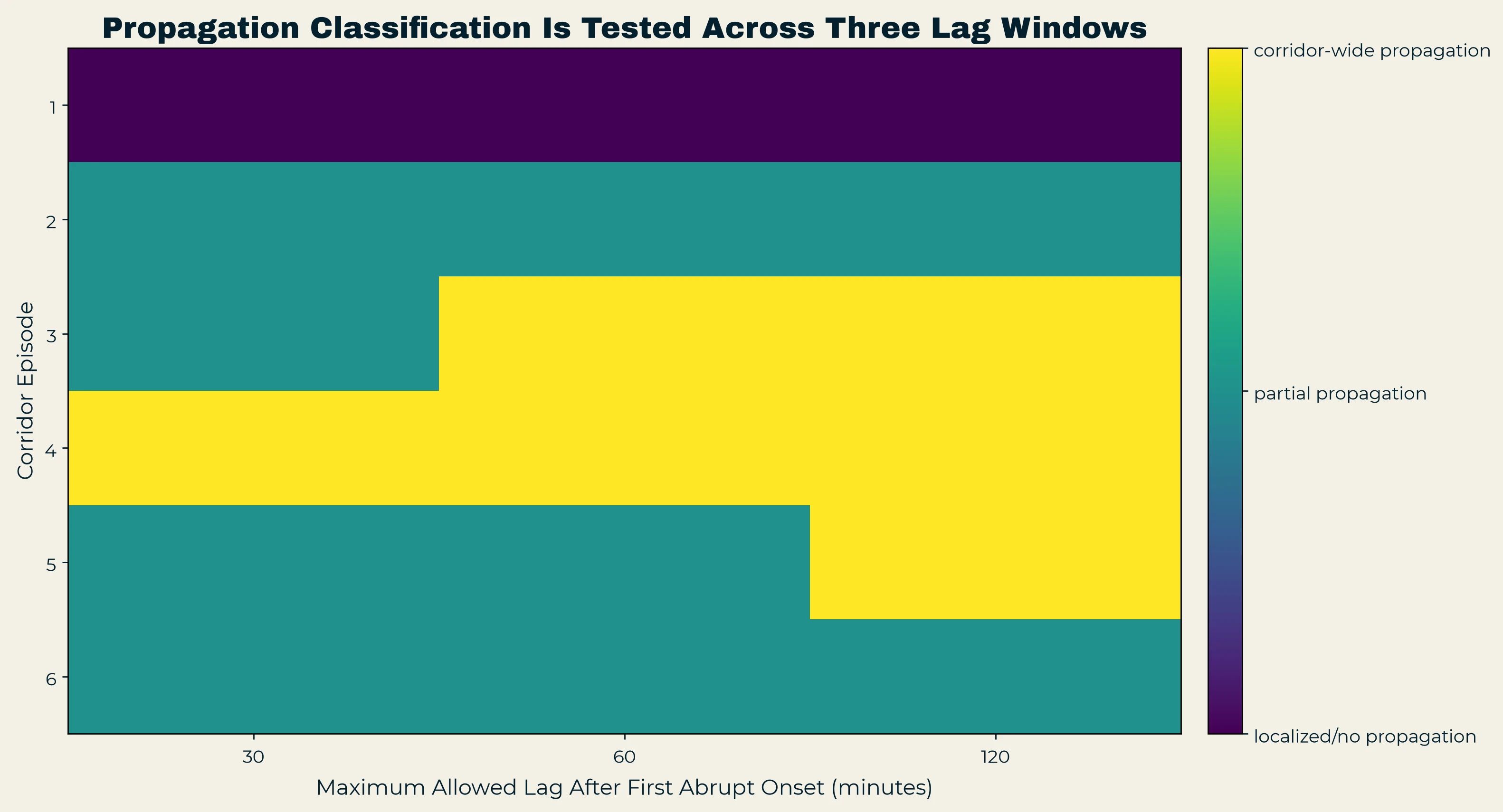
Some episodes add congested stations quickly, others take much longer, and some stations never enter the sustained state within the window (Figures A6 and A7). If every episode propagated neatly along the direction of travel, the station-entry lags would share an ordered progression, and they do not. Episode 4 comes closest to a corridor-wide pattern within a short interval, while the other episodes involve only part of the detector chain or bring stations in much later.
The classification therefore depends partly on how long the analysis waits after the first onset. I tested maximum participation windows of 30, 60 and 120 minutes. Figure 8 shows the number of participating stations in each episode under each window. Episodes 1, 2, 4 and 6 are stable across the tested windows and keep the same basic classification (Figure A8). Episode 3 eventually adds another station, and Episode 5 expands from three participating stations to all five only under the longest window.
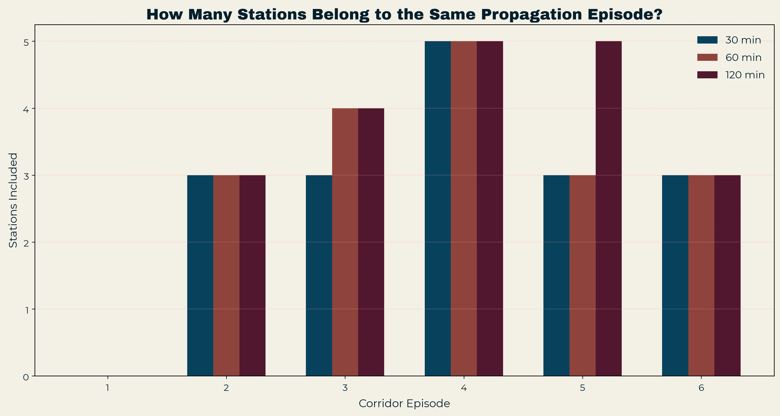
The propagation result is descriptive. Some breakdowns stay local, some involve several stations quickly, and others recruit stations over a much longer period, and the episode grid shows that variation before any summary number does.
Duration
How Long Sustained Congestion Lasts
The abrupt-drop sample contains only ten events, so duration is better studied with the 1,457 sustained congestion events. The distribution is strongly right-skewed, with an overall median of about 60 minutes and a 90th percentile of about 355 minutes.
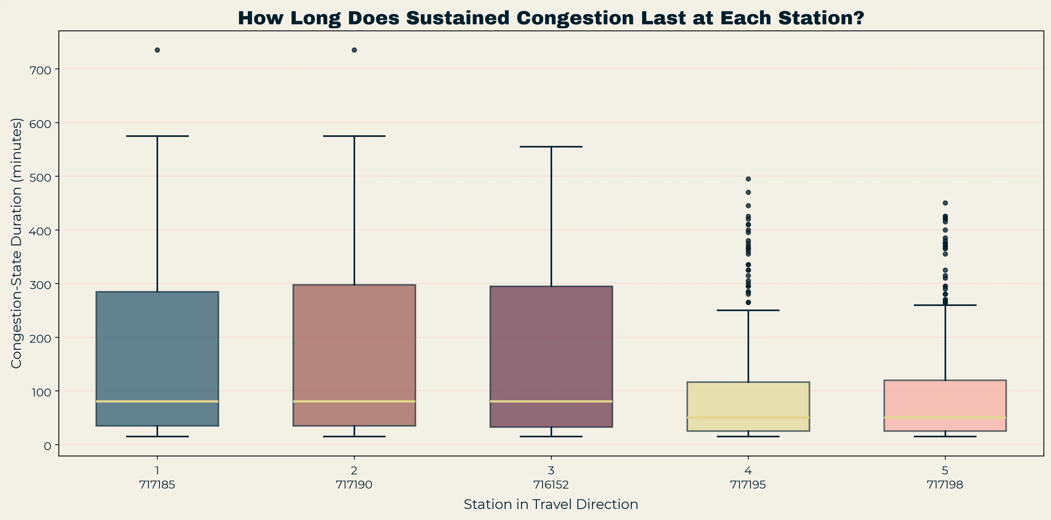
Station location matters. Figure 9 compares duration across the five stations. The three upstream stations have medians around 80 minutes, while the two downstream stations near Azusa are closer to 50 minutes, the same split around the Lark Ellen to Azusa 1 bottleneck described above. Long episodes occur at every station, but the distributions differ.
The larger difference appears when events are grouped by start time. Episodes beginning between 10:00 and 14:59 last much longer than those beginning in the morning or late afternoon.
One concern is that this could be an artifact of the event rule. If speed rises above 50 mph for five minutes and then falls back, that brief recovery splits one traffic episode into two. I repeated the duration calculation while merging gaps of 0, 5, 10 and 15 minutes. The merge test re-detects events on the full day of data rather than the original analysis window, so it starts from 1,462 events instead of 1,457.
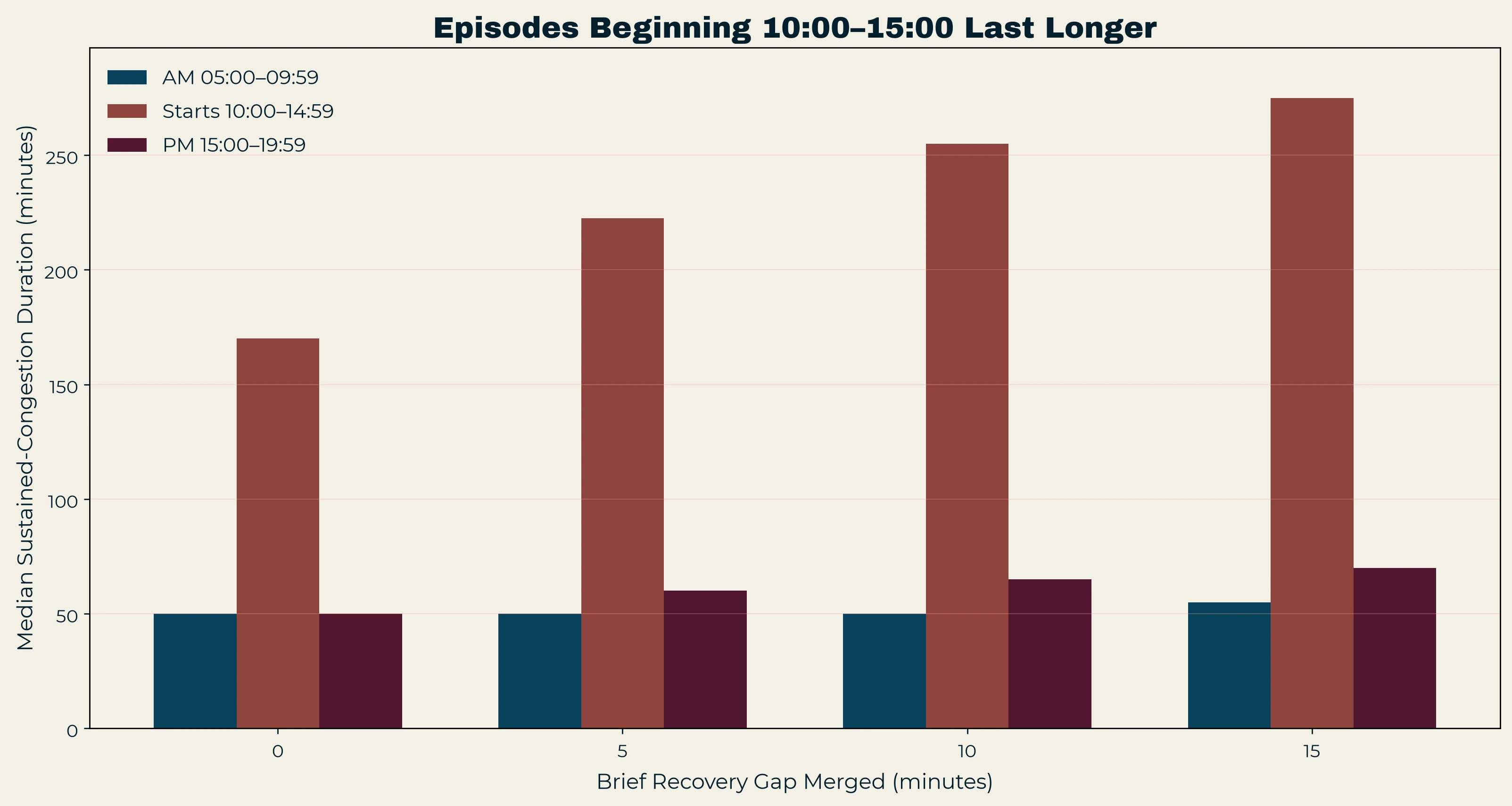
Figure 10 shows the result. With no merging, the median duration for episodes beginning from 10:00 through 14:59 is about 170 minutes, while morning and late-afternoon starts are around 50 minutes. Merging five-minute gaps raises the 10:00 to 14:59 median above 220 minutes, a ten-minute allowance brings it to around 255, and a fifteen-minute allowance brings it close to 275. The morning and late-afternoon medians move much less. The direction of the result does not depend on treating every short recovery as the end of an episode.
| Gap merged | Median duration |
|---|---|
| None | about 170 min |
| 5 minutes | above 220 min |
| 10 minutes | about 255 min |
| 15 minutes | about 275 min |
Part of the explanation is visible in the same test. Sixty-one percent of episodes that began between 10:00 and 14:59 were still congested at 15:00, rising to 71 percent with the 15-minute merge. Most of these episodes start before 3 p.m. and run into the afternoon. The accurate claim is about start-time groups: episodes beginning from roughly 10:00 through 15:00 lasted longer on this corridor during the study period. I would not restate that as “midday congestion lasts longer,” because the data classify episodes by when they begin and do not establish a midday effect.
Influence checks
The Duration Result Is Not Coming From One Detector or One Day
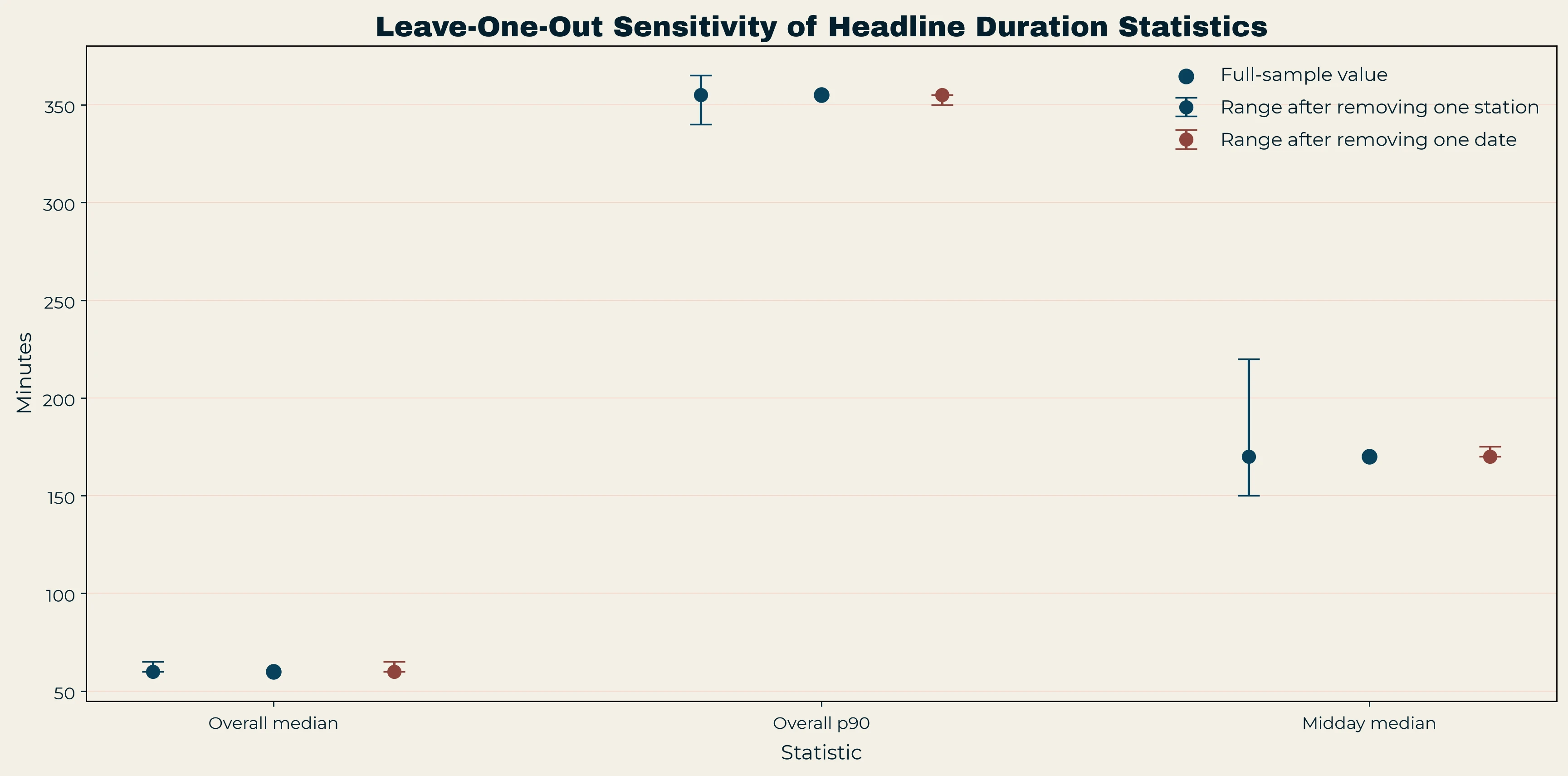
A pattern in observational traffic data can be driven by one unusual station or one bad day. Figure 11 compares the full-sample values with the ranges produced by removing one station at a time and one date at a time. The overall median stays close to 60 minutes and the 90th percentile close to 355 minutes. The median for episodes starting 10:00 to 14:59 moves more when individual stations are removed, but it never falls to the morning level, and removing individual dates produces a much narrower range. The start-time finding survives both forms of leave-one-out testing, while the station-level range shows that its exact size should not be treated as fixed.
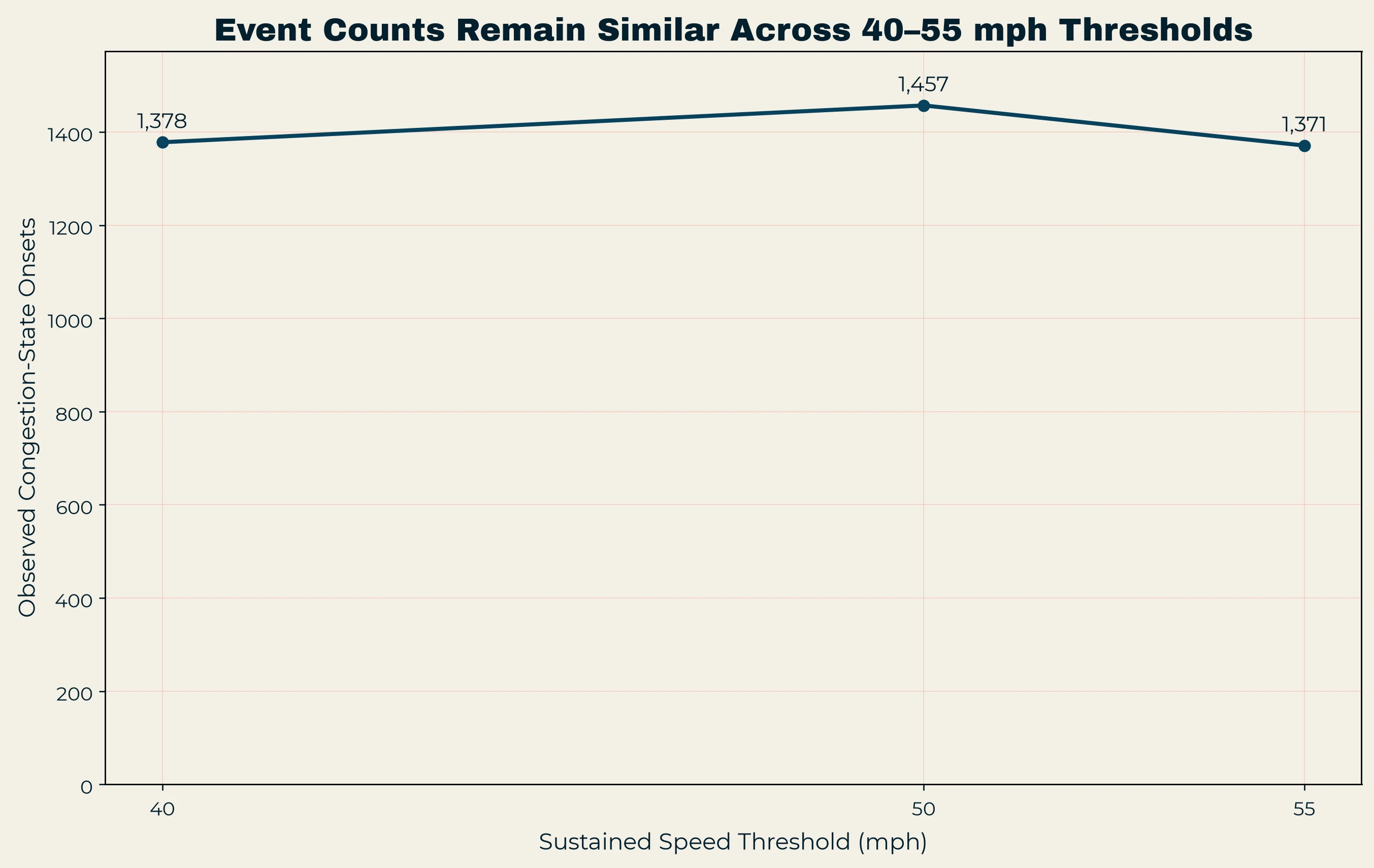
The sustained-state count was also checked against the speed threshold itself, using the 40 and 55 mph ends of FHWA’s breakdown range (FHWA-HOP-19-029). Thresholds of 40, 50 and 55 mph give 1,378, 1,457 and 1,371 events. Changing the threshold within this range does not produce a very different number of congestion onsets, so the main inventory is not the product of one convenient cutoff (Figure A9).
Recovery
Recovery Is Less Orderly Than Formation
If congestion always formed in one direction and cleared in reverse, recovery would be simple to describe, and the observed episodes do not behave that way. Figure 12 plots recovery timing across stations for the corridor episodes. Some episodes recover earlier upstream, others earlier downstream, and a few stations recover at nearly the same time despite different onset histories.
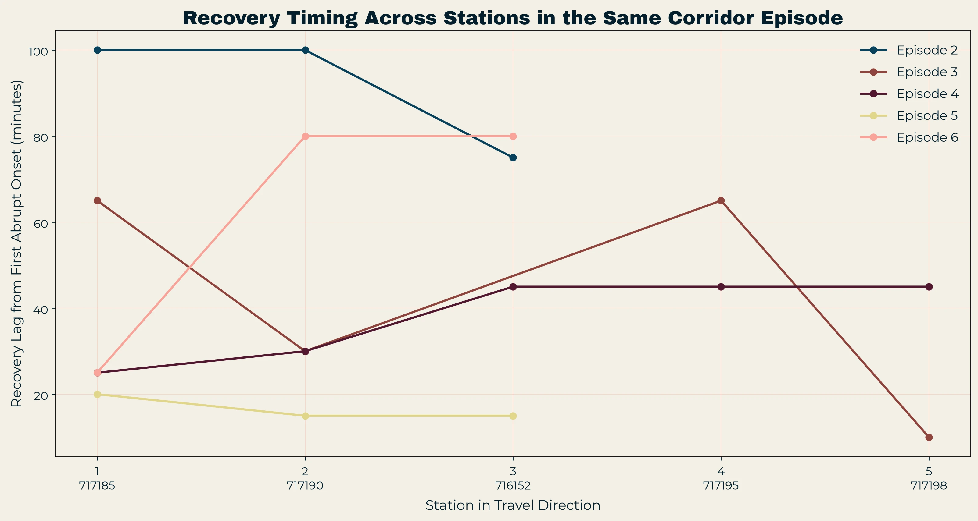
The station-order correlations change sign from episode to episode. Recovery lag rises with station order in Episodes 4 and 6 and falls with it in Episodes 2, 3 and 5. Each correlation rests on three to five stations, so the signs mean more than the magnitudes. FHWA describes recurring bottlenecks as clearing from the rear of the queue as volume declines, while nonrecurring bottlenecks can clear from either end depending on the cause (FHWA-HOP-18-013). A mix of recovery directions is what one would expect if these episodes do not share a single mechanism, and there is no defensible single recovery direction for this corridor.
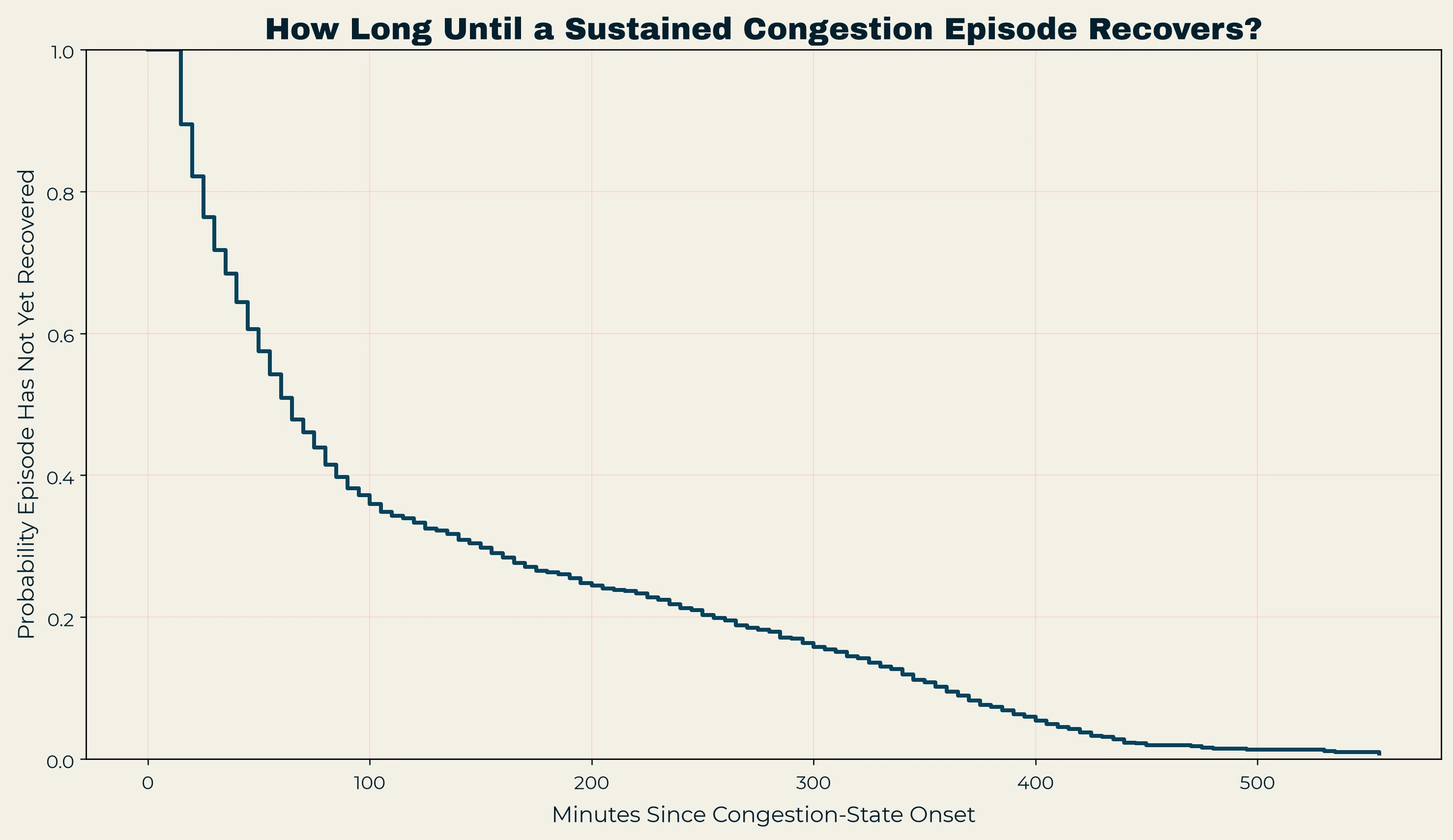
The full sustained-event sample gives another view. Figure 13 plots the share of congestion episodes that have not yet recovered as time passes. Sixty-two episodes were still congested when the observable record ended, so their true durations are unknown. The Kaplan–Meier estimator keeps them in the calculation as right-censored observations rather than treating their last observed time as a recovery (Kaplan and Meier, 1958). The curve falls quickly during the first hour and then develops a long tail, with a sizeable minority of episodes still active after one to two hours and a small number lasting several hundred minutes.
The two recovery figures answer different questions. The episode plot asks where recovery happens first within a particular corridor event, and the survival curve asks how long sustained congestion stays unresolved across the whole inventory. A single median could not describe either one.
Revisions
What Changed While the Analysis Was Being Challenged
Several parts of the project were revised after the first calculations.
The corridor changed. An early ranking favored a longer I-210 West run, and the final selection moved to this I-10 section after candidates were ranked by weakest-station coverage and recurring low-speed traffic.
The control comparison changed materially. The first matched controls included intervals that were already congested, which raised control occupancy enough to make event occupancy look slightly lower. Restricting the controls to free-flow conditions reversed the sign. In the corrected comparison, flow five minutes before onset is nearly the same in both groups, while the event observations have lower speed and higher occupancy.
Event 340 changed another interpretation. Looking one interval back classified all ten events as starting above 50 mph. The wider t−30 to t−10 window showed that 340 was already congested, and placing it at Azusa 2 tied it to the downstream origin of Episode 3.
The clustering claim was dropped. The six episodes are six calendar dates, so no clustering result could have come out of them. Propagation sensitivity is a separate question, and there four of six episodes keep their classification across the tested windows.
A breakdown probability calculation was dropped from the presentation. The product-limit method for estimating breakdown probability from censored observations is well established (Brilon et al., 2005), but with only ten abrupt events the estimate said little beyond the fact that the rule identifies rare events. Flows measured at stations already inside an upstream queue also reflect queue discharge rather than demand, which weakens the flow values the method depends on.
The source of the abrupt-drop thresholds was corrected. The 20 mph and 40 mph values were first attributed to a temporal rule in the SHRP2 C05 report. Tracing the report’s citation led to Chen et al. (2004), where the thresholds define a spatial comparison between upstream and downstream detectors (SHRP2 C05; Chen et al., 2004). The rule itself was kept exactly as implemented and is now described as this project’s adaptation of those thresholds.
None of these revisions changed the abrupt-drop rule after the results were seen. The ten-event inventory stays fixed, and the persistence and pre-window tests are reported as sensitivity checks around it.
Conclusions
What I Would Claim From This Corridor
The study covers one short segment of one freeway over four months. The abrupt-drop sample contains ten events, four of them on the same date, so several conclusions apply only to this corridor and this period.
Within those limits, sustained congestion and abrupt onset are clearly different measurements. The 50 mph sustained-state rule identifies 1,457 events, the abrupt-drop rule 10, and the Caltrans spatial rule 7. Those counts are too far apart for the definitions to substitute for one another.
Seven of the ten abrupt drops fit the strongest version of the breakdown story used here: they begin in free flow and stay below 40 mph afterward. Events 1 and 346 begin in free flow but recover quickly, and event 340 is an abrupt drop inside traffic that was already congested.
Five minutes before the ten abrupt drops, median speed is lower than in matched free-flow controls, occupancy is higher, and flow is almost unchanged. Occupancy rises from 0.0747 at t−10 to 0.1088 at t−5, so in this sample the measurable change is concentrated very close to the collapse, and part of it may fall inside the collapse interval itself.
The strongest recurring bottleneck signal lies between Lark Ellen and Azusa 1, and the longer congestion durations at the three stations upstream of it are consistent with a queue forming behind that point. The corridor is too short to show that every disturbance starts there, and one episode appears to enter from the downstream boundary.
The six episodes do not share one propagation pattern. Four keep their classification when the propagation window changes, and two do not.
The larger sustained-congestion sample gives the clearest duration result. Episodes beginning from 10:00 through 14:59 last substantially longer than morning or late-afternoon starts, the difference holds when short recoveries of 5, 10 and 15 minutes are merged, and most of those episodes are still congested at 15:00. Recovery has no common station order.
These are modest claims about one corridor. What the project offers is a measured distinction between the low-speed state and the transition that creates it, along with a short list of patterns that held up when I tried to break them.
Supporting figures
Appendix: Supporting Figures
These figures support checks described in the text. They are kept here so the main narrative stays focused on the findings.
Source
Repository
The analysis script, audit outputs and every figure are in the repository.
Sources
References
- Bertini, R. L., and Myton, A. M. (2005). Use of Performance Measurement System data to diagnose freeway bottleneck locations empirically in Orange County, California. Transportation Research Record, 1925, 48–57.
- Brilon, W., Geistefeldt, J., and Regler, M. (2005). Reliability of freeway traffic flow: A stochastic concept of capacity. In Transportation and Traffic Theory: Proceedings of the 16th International Symposium on Transportation and Traffic Theory, 125–144.
- California Department of Transportation. PeMS bottleneck identification documentation. [URL and access date to add]
- Cassidy, M. J. (1998). Bivariate relations in nearly stationary highway traffic. Transportation Research Part B, 32(1), 49–59.
- Cassidy, M. J., and Bertini, R. L. (1999). Some traffic features at freeway bottlenecks. Transportation Research Part B, 33(1), 25–42.
- Chen, C., Petty, K., Skabardonis, A., Varaiya, P., and Jia, Z. (2001). Freeway performance measurement system: Mining loop detector data. Transportation Research Record, 1748, 96–102.
- Chen, C., Kwon, J., Rice, J., Skabardonis, A., and Varaiya, P. (2003). Detecting errors and imputing missing data for single-loop surveillance systems. Transportation Research Record, 1855, 160–167.
- Chen, C., Skabardonis, A., and Varaiya, P. (2004). Systematic identification of freeway bottlenecks. Transportation Research Record, 1867, 46–52.
- Chow, A. H. F., Lu, X.-Y., and Qiu, T. Z. (2009). An empirical analysis of freeway traffic breakdown probability based on bivariate Weibull distribution. IFAC Proceedings Volumes, 42(15), 472–477.
- Chung, K., Rudjanakanoknad, J., and Cassidy, M. J. (2007). Relation between traffic density and capacity drop at three freeway bottlenecks. Transportation Research Part B, 41(1), 82–95.
- Daganzo, C. F., Cassidy, M. J., and Bertini, R. L. (1999). Possible explanations of phase transitions in highway traffic. Transportation Research Part A, 33(5), 365–379.
- Federal Highway Administration. FHWA-HOP-08-054, Section 6. [Title and year to confirm]
- Federal Highway Administration. Recurring Traffic Bottlenecks: A Primer. FHWA-HOP-18-013. [Edition and year to confirm]
- Federal Highway Administration. FHWA-HOP-19-029, Chapter 4. [Title and year to confirm]
- Kaplan, E. L., and Meier, P. (1958). Nonparametric estimation from incomplete observations. Journal of the American Statistical Association, 53(282), 457–481.
- Lighthill, M. J., and Whitham, G. B. (1955). On kinematic waves II. A theory of traffic flow on long crowded roads. Proceedings of the Royal Society of London, Series A, 229(1178), 317–345.
- Lorenz, M. R., and Elefteriadou, L. (2000). A probabilistic approach to defining freeway capacity and breakdown. In Transportation Research Circular E-C018: Fourth International Symposium on Highway Capacity, 84–95. Transportation Research Board.
- PeMS field specification, Station 5-Minute data. Reproduced in a SHRP2 report appendix. [Report number to confirm, or replace with the PeMS page]
- Persaud, B., Yagar, S., and Brownlee, R. (1998). Exploration of the breakdown phenomenon in freeway traffic. Transportation Research Record, 1634, 64–69.
- Rajagopal, R., and Varaiya, P. (2007). Health of California’s Loop Detector System (UCB-ITS-PRR-2007-13). California PATH Program, University of California, Berkeley.
- Transportation Research Board. Understanding the Contribution of Operations, Technology, and Design to Meeting Highway Capacity Needs (SHRP2 Report S2-C05-RW-1), §2.3.3, p. 2-5. [Title and year to confirm]